L30 - CFAR Processing#
CFAR Processing
A threshold set from 32 neighboring cells holds one false alarm in a million at any noise level, losing 1 dB of SNR.
Lesson 30 · Antennas, Phased Arrays, and Radar Systems · Dr. Neil Rogers
Printing
To print the slides, switch to present mode and print: one slide a sheet, with room for notes. Print from read mode for the whole lesson.
Learning Objectives
- I can apply constant false-alarm rate (CFAR) processing to radar data and evaluate detection performance.
Lesson 27 set a detection threshold from the probability of false alarm, assuming the processor knows the noise power, and ended by showing what happens when it does not. This lesson replaces the assumed noise power with one measured from the data around each cell. That is constant false-alarm rate (CFAR) processing, and it is the detector you will run on your own range-Doppler maps from Lesson 29.
You work the L28–L31 Labs outside class, so this page carries the whole argument in read mode. The lesson comes first; the L30 Lab follows it on this page.
A Moving Noise Floor
A fixed threshold assumes the noise power \(P_n\) is known.
3 dB more noise turns \(P_{fa} = 10^{-6}\) into \(10^{-3}\).
CFAR measures \(P_n\) around each cell it tests.
Lesson 27 found that noise power in one cell is exponentially distributed with mean \(P_n\), so noise alone crosses a threshold \(T\) with probability
The threshold for \(P_{fa} = 10^{-6}\) is \(T = 13.8\ P_n\), 11.4 dB above the mean noise. If the noise rises by a factor \(g\) while \(T\) stays put, the probability becomes \(P_{fa}^{1/g}\), and a 3 dB rise turns \(10^{-6}\) into \(10^{-3}\). At the half a million decisions a second of the L29 burst, that is 500 false targets a second.
The noise on a real map does move. Stationary clutter fills the cells near zero velocity, strong reflections fill the cells nearest the radar, and the receiver gain sets the level of everything. A fixed threshold high enough for the worst of these misses targets everywhere else. Lesson 27’s last figure showed the alternative: estimate the noise power from the cells around the one being tested, and set the threshold from that estimate.
Cell Under Test, Guard, and Reference
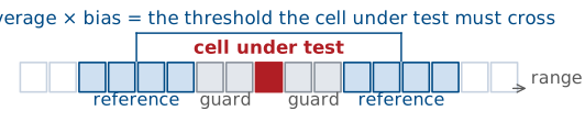
Reference cells estimate the local noise.
Guard cells keep the target’s own energy out of the estimate.
The window slides, so every cell gets its own threshold.
The detector tests one cell at a time, the cell under test. On each side of it, it skips a few guard cells and then averages a block of reference cells. The average is the estimate of the noise power at this cell, and the threshold is that estimate multiplied by a bias. If the cell under test exceeds the threshold, the detector declares a target there. Then the window moves one cell and the detector repeats the test, so the detector recomputes the threshold at every cell from that cell’s own neighbors.
The figure draws 2 guard and 4 reference cells a side so that the cells are readable. The running example in this lesson uses 2 guard and 16 reference cells a side, \(N = 32\) reference cells in all, which is the local-average threshold in Lesson 27’s last figure. ADI’s CFAR lab lists the same steps for the PHASER: pick the cell, skip the guard cells, average the reference cells, multiply by the bias, and compare.
Cell-Averaging CFAR
\(P_{fa}\) depends on \(\alpha\) and \(N\), and not on \(P_n\).
With \(z_i\) the power in reference cell \(i\), the cell-averaging (CA) CFAR estimate of the noise power is the sample mean \(\hat{P}_n\), and the threshold is \(T = \alpha\hat{P}_n\). The bias \(\alpha\) is the number we choose.
For a given estimate, the cell under test crosses the threshold with probability \(e^{-T/P_n}\), the Lesson 27 result. The estimate is itself random, so the probability of false alarm is the average of that over the reference cells. Each \(z_i\) is independent and exponential with mean \(P_n\), and for one such cell the average of \(e^{-cz_i/P_n}\) is \(1/(1 + c)\). The exponential of a sum is a product, so
where the angle brackets mean the average over the noise. \(P_n\) has dropped out. Wherever the noise sits, whether 0 dB or 15 dB, the probability that noise alone crosses the threshold is the same, which is what constant false-alarm rate means. Two assumptions came with it: the reference cells hold only noise, and their noise has the same mean as the noise in the cell under test. The rest of the lesson is about what happens when either one fails.
The Bias From the False-Alarm Probability
A known \(P_n\) needs 11.4 dB; 32 reference cells need 12.4 dB.
Inverting the false-alarm expression gives the bias for a chosen \(P_{fa}\):
For \(P_{fa} = 10^{-6}\) and \(N = 32\), \(\alpha = 32(10^{6/32} - 1) = 17.3\), or 12.4 dB. With 16 reference cells it is 21.9, 13.4 dB; with 144 it is 14.5, 11.6 dB. As \(N\) grows,
which is the 11.4 dB threshold of Lesson 27, because an average over infinitely many cells equals the noise power.
The bias is larger with fewer cells because the estimate scatters. Sometimes it comes out low, the threshold drops with it, and noise crosses more often than it would with the true \(P_n\). Raising \(\alpha\) compensates for those low estimates. In the code later in this lesson, bias_db is \(10\log_{10}\alpha\).
Note
ADI’s target_detection_dbfs.py averages the reference cells in dB and adds the bias in dB. That is a different estimator: the average of \(10\log_{10}z\) over exponential noise sits 2.5 dB below \(10\log_{10}P_n\), so a bias in ADI’s code is not the \(\alpha\) of this lesson. Its threshold still follows the noise, so it is still a CFAR, but this lesson’s numbers do not apply to it. Read ADI’s code beside the provided cfar_2d, which averages power.
CFAR Loss
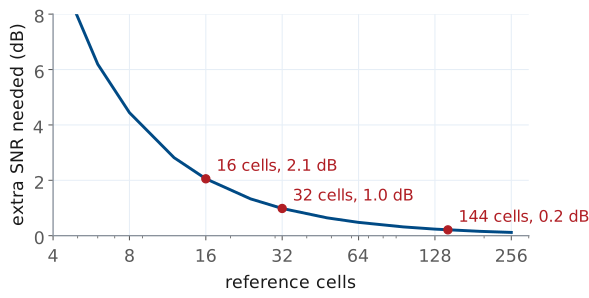
A higher bias needs more SNR for the same \(P_d\).
32 cells lose 1.0 dB; 16 lose 2.1 dB.
More cells lose less, until the window reaches noise of a different level.
A target that a known-noise detector finds with \(P_d = 0.9\) at \(P_{fa} = 10^{-6}\) needs 13.2 dB of SNR (Albersheim’s fit in Lesson 27 gave 13.1 dB). The CA-CFAR detector needs more, because its threshold is higher on average and scatters with the estimate. The difference is the CFAR loss. The figure computes it by averaging the Lesson 27 detection probability over the scatter of \(\hat{P}_n\): 2.1 dB with 16 reference cells, 1.0 dB with 32, and 0.2 dB with 144.
The figure favors many reference cells, but a wider window is more likely to reach noise of a different level. The estimate assumes that every reference cell has the same mean noise as the cell under test. A window 32 cells wide in range spans 9.6 m at the 0.30 m cells of the L29 burst, and the clutter near the radar does not stay level over 9.6 m. The number of reference cells trades the CFAR loss against how local the estimate is.
Choosing the Guard Cells
A Hann window puts −6 dB of the target in each neighboring cell.
Without guard cells, the target raises its own threshold.
Guard cells cover the target’s extent, in range and in Doppler.
A target does not occupy exactly one cell. The window applied before the FFT, Hann in ADI’s scripts and in the L29 range-Doppler map, widens the target’s peak so that each neighboring cell holds a quarter of its power, 6 dB down. A person is also larger than one 0.30 m range cell, and moving arms and legs spread the echo over several Doppler cells.
Without guard cells, that spill lands in the reference cells. Take a 20 dB target with no guard cells and 32 reference cells. Its two neighbors hold 14 dB each, 25 times the noise power, and they raise the estimate from \(P_n\) to about \((30 + 2 \times 26)/32 = 2.6\ P_n\), which lifts the threshold by 4.1 dB. The target still crosses, but its margin shrinks from 7.6 dB to 3.5 dB, and a weaker target would not. One or two guard cells a side remove the problem. More guard cells than the target’s extent do no harm to the target, but they push the reference cells farther out, where the noise is less likely to match.
CFAR Explorer
The widget draws one range profile of 240 cells, in dB, with the CFAR threshold over it in green. Cells from 168 on hold clutter 15 dB above the quiet noise. Triangles along the top mark five targets, each with the Hann window’s −6 dB neighbors, dark when found and pale when missed: a pair eight cells apart near cell 56, one alone near 104, one in the clear just short of the clutter at 160, and one inside the clutter. Found targets are ringed; noise crossings are red dots, and the widget counts them as false alarms. The readout gives the design \(P_{fa}\) for the method, bias, and number of reference cells.
Start at 2 guard and 16 reference cells a side with a 12.4 dB bias, the lesson’s running example. Set the guard cells to 0 and watch each target lift its own threshold. Lower the bias until false alarms appear, and compare where they appear with the design \(P_{fa}\). Then switch the method to greatest-of and smallest-of, the subject of the next frames, and press New noise for another draw of the same scene.
Failures of Cell Averaging
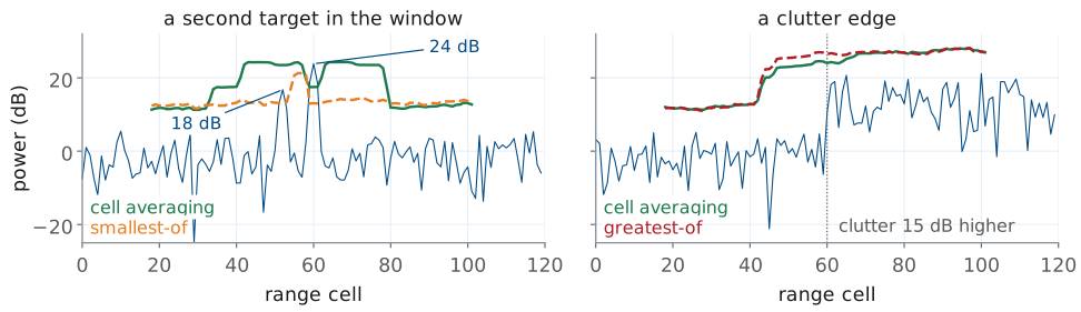
A second target in the window hides the weaker one: masking.
At a clutter edge, one average mixes two noise levels.
Cell averaging assumes that every reference cell holds noise of the same mean as the cell under test. The figure shows the two common ways that fails.
On the left, an 18 dB target sits eight cells from a 24 dB target. When the weaker target is the cell under test, the stronger one and its two neighbors are in its reference window, and they hold about \(251 + 2 \times 63\) times the noise power. Spread over 32 cells, that raises the estimate by a factor of about 12.7, 11 dB, so the threshold rises to 23.5 dB and the detector misses the 18 dB target. This is masking, and it happens wherever targets are close together: two people walking side by side, or a hand in front of a body.
On the right, the noise rises 15 dB at cell 60, the edge of a clutter region. A cell in the clear just before the edge has half its reference cells in the clutter, so its threshold rises by about 12 dB and a target there is masked. A cell in the clutter just past the edge has half its reference cells in the clear, so its estimate is half what it should be, the threshold sits 3 dB low, and its \(P_{fa}\) rises from \(10^{-6}\) to \((1 + \alpha/32)^{-16} = 10^{-3}\). The clutter edge produces false alarms on one side and misses on the other.
Greatest-Of and Smallest-Of
Greatest-of holds \(P_{fa}\) at a clutter edge.
Smallest-of finds a target beside another.
Each needs its own bias, and loses 0.2 or 0.7 dB more than cell averaging.
Both variants average the two sides of the window separately, \(\hat{P}_\text{near}\) over the reference cells nearer the radar and \(\hat{P}_\text{far}\) over those farther away, and then keep one of the two.
Greatest-of (GO) keeps the larger. At a clutter edge, the side in the clutter wins, so GO compares a cell just inside the clutter with the clutter level, and its false alarms stay near the design value; the dashed red line in the right panel of the last figure does that. GO misses targets in the clear cells just before the edge, which it also compares with the clutter, and it makes masking worse.
Smallest-of (SO) keeps the smaller. When a second target sits on one side, the clean side wins and the weaker target is found, as the dashed orange line in the left panel shows. SO fails at clutter edges instead, where it takes the quiet side and lets the clutter through.
Neither max nor min of two averages is an average, so each has its own relation between \(\alpha\) and \(P_{fa}\). With 16 cells a side and \(P_{fa} = 10^{-6}\), GO needs a bias of 12.0 dB on its larger half and SO 13.7 dB on its smaller half, against 12.4 dB for CA. For \(P_d = 0.9\), GO needs 0.2 dB more SNR than CA and SO 0.7 dB more. ADI’s cfar() takes the three methods as 'average', 'greatest', and 'smallest'; the widget switches among them.
The Ends of the Map
The first and last range cells have reference cells on one side only.
One-sided with the same bias, \(P_{fa}\) rises from \(10^{-6}\) to \(8 \times 10^{-6}\).
Doppler wraps: the cell past +15 m/s is −15 m/s.
The window runs out at the ends of the data. In range, a cell within \(g + n\) of the first or last cell has fewer reference cells on one side, or none. There are three choices: skip those cells and never declare a detection there; average whatever reference cells exist, which is what this lesson’s code does; or raise the bias for the cells with fewer neighbors. With the second choice, 16 reference cells instead of 32, and the bias left at 12.4 dB, \(P_{fa}\) rises to \((1 + 17.3/16)^{-16} = 8 \times 10^{-6}\), a small increase that keeps those cells in the test. The one choice to avoid is padding with zeros and counting them, which drags the estimate down and the false alarms up. ADI’s cfar() does not test the end cells against their own neighbors: it gives them the lowest threshold found anywhere in the profile, so a strong return near either end is reported whatever the noise around it. The cells nearest 0 m on the PHASER hold the kit’s own transmit-to-receive leakage, so they are usually excluded in any case.
Doppler is different. The Doppler FFT is periodic: the cell above the highest velocity, +15 m/s for the L29 burst, is the lowest, −15 m/s. A reference window that runs off one end of the Doppler axis continues at the other, so it never runs out, and the Doppler edge needs no special case.
2D CFAR on the Range-Doppler Map
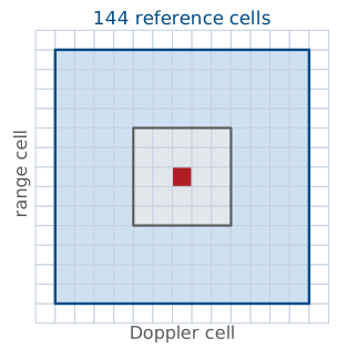
The guard and reference cells become nested boxes.
2 guard and 4 reference cells each way give 144 cells: 11.6 dB, 0.2 dB loss.
The zero-velocity clutter ridge is an edge: run MTI first.
The range-Doppler map has two axes, so the window does too. The guard cells become a box around the cell under test, and the reference cells are the ring between that box and a larger one. With 2 guard and 4 reference cells each way from the cell under test, in both range and Doppler, the outer box is 13 by 13 cells and the guard box 5 by 5, so \(N = 169 - 25 = 144\). The bias for \(P_{fa} = 10^{-6}\) is 11.6 dB and the CFAR loss is 0.2 dB, far better than any one-dimensional window can do while staying within a few cells of the cell under test.
The two directions need not match. At the L29 burst’s 0.30 m range cells and 0.12 m/s velocity cells, a walking person spans a cell or two in range but many cells in Doppler, because the arms and legs move at different speeds from the body. A wider guard band in Doppler than in range keeps that spread out of the estimate.
Without MTI, every stationary object puts its echo at zero velocity, so the map has a ridge of clutter along the zero-Doppler column. To a CFAR window, that ridge is a clutter edge in the Doppler direction: cells on the ridge are compared with an average that is mostly noise, and they are declared targets. MTI from Lesson 29 removes most of the ridge before CFAR runs.
The L29 burst’s map of \(269 \times 256\) cells, with 144 reference cells each, is 10 million additions. A Python loop over every cell is slow, but a convolution of the map with the window does the same sums in a fraction of a second, and the next frame’s code works that way.
Detections From the Map
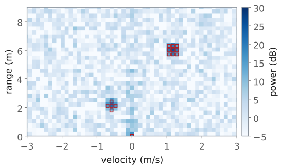
The provided
cfar_2dreturns a detection map and a list of (range, velocity, SNR).One target produces a cluster of detections.
CFAR also detects the clutter that MTI leaves.
The map is synthetic, built with the L29 burst’s cells: a walker at 6.0 m and +1.2 m/s, a hand at 2.1 m and −0.6 m/s, and the clutter a 2-pulse canceller leaves at zero velocity near the radar. CFAR with 2 guard and 4 reference cells each way and an 11.6 dB bias declares both targets and the strongest clutter cell. Each target produces a cluster of detections, because its peak spreads into its neighbors and those neighbors are well above the noise too. A detection list that feeds a classifier or a tracker needs one entry per object, so we reduce each cluster to its strongest cell.
The excerpt is the cell-averaging path of the provided cfar_2d in radar_lab.py, which the L30 Lab notebook calls; the provided version also takes method="ca", "go", or "so" for the variants above. It takes the map in dB, as Lesson 29 plots it, and converts it back to power, because the CFAR statistics of this lesson are for power. guard and ref are (range, Doppler) pairs of half-widths. The two convolutions sum each cell’s reference window and count how many cells it held, so an end cell in range averages only the cells that exist; the code wraps the Doppler axis. Pass the map’s axes, and the detection list comes back in meters and meters per second.
import numpy as np
from scipy import signal
def cfar_2d(rd_map, guard, ref, bias_db, axes=None):
    P = 10 ** (rd_map / 10)                                  # dB back to power
    (gr, gv), (rr, rv) = guard, ref                          # (range, Doppler) half-widths
    win = np.ones((2 * (gr + rr) + 1, 2 * (gv + rv) + 1))
    win[rr:rr + 2 * gr + 1, rv:rv + 2 * gv + 1] = 0          # guard cells and the cell under test
    def pad(A): return np.pad(np.pad(A, ((0, 0), (gv + rv,) * 2), "wrap"), ((gr + rr,) * 2, (0, 0)))
    total = signal.fftconvolve(pad(P), win, mode="valid")
    count = signal.fftconvolve(pad(np.ones_like(P)), win, mode="valid")
    snr_db = 10 * np.log10(P / (total / count))              # each cell over its local noise
    det = snr_db > bias_db
    r_ax, v_ax = axes or (np.arange(P.shape[0]), np.arange(P.shape[1]))
    hits = [(r_ax[i], v_ax[j], snr_db[i, j]) for i, j in zip(*np.nonzero(det))]
    return det, hits
The SNR in each entry is the cell’s power over its own local noise estimate, the same quantity the threshold tests, so it is the number to compare with Lesson 27.
Measuring the False-Alarm Rate
At \(10^{-6}\), a \(269 \times 256\) map averages one false alarm every 15 maps.
Check the design at a lower bias, where false alarms are common.
\(P_d\) is the fraction of maps that find the target.
We set the bias from a design \(P_{fa}\) and check it by counting. On maps with no target, or in the cells far from any target, every detection is a false alarm, and the measured probability is the number of false detections over the number of cells tested.
Counting false alarms at the design rate takes many maps: the L29 burst’s map of \(269 \times 256\) cells is 68 864 decisions, so at \(10^{-6}\) it averages 0.07 false alarms, one every 15 maps. Counting ten of them to get the rate within about a third takes 145 maps. Instead, we lower the bias to a design \(P_{fa}\) of \(10^{-3}\) or \(10^{-4}\), where a single map has 7 to 69 false alarms, and check the measured rate against \((1 + \alpha/N)^{-N}\) at a few biases. If the counts follow the curve, the extrapolation to \(10^{-6}\) is sound; if they come out high, the noise in the reference cells does not match the noise in the cells under test.
We measure the probability of detection the same way, against a target you placed: the fraction of maps in which CFAR declares it. Compare it with Lesson 27’s curves at the SNR the detection list reports, with the CFAR loss added. For a hand or a person, which fluctuate from map to map, expect the Swerling numbers of Lesson 27 rather than the steady ones.
Summary
Symbol / idea |
What it is |
Number to remember |
|---|---|---|
Fixed threshold, noise up by \(g\) |
\(P_{fa}' = P_{fa}^{1/g}\) |
3 dB: \(10^{-6} \to 10^{-3}\) |
Cell under test, guard, reference |
test one cell; skip its neighbors; average the next ones |
2 guard and 16 reference cells a side |
CA-CFAR |
\(T = \alpha\hat{P}_n\), \(P_{fa} = (1 + \alpha/N)^{-N}\) |
independent of \(P_n\) |
Bias |
\(\alpha = N(P_{fa}^{-1/N} - 1)\) |
12.4 dB for 32 cells at \(10^{-6}\); 11.4 dB as \(N \to \infty\) |
CFAR loss |
extra SNR for the same \(P_d\) |
2.1 dB at 16 cells, 1.0 dB at 32, 0.2 dB at 144 |
Guard cells |
keep the target’s spread out of the estimate |
Hann: −6 dB one cell away |
Masking |
a second target raises the threshold |
24 dB eight cells away hides 18 dB |
Clutter edge |
one average over two noise levels |
\(P_{fa}\) to \(10^{-3}\) just inside the clutter |
Greatest-of, smallest-of |
keep the larger or smaller half |
GO for edges, SO for close targets; 0.2 and 0.7 dB more loss |
Ends of the map |
range: one-sided; Doppler: wraps |
one-sided at the same bias: \(8 \times 10^{-6}\) |
2D CFAR |
nested boxes on the range-Doppler map |
144 cells: 11.6 dB, 0.2 dB loss |
Measured \(P_{fa}\) |
false detections over cells tested |
\(10^{-6}\) on \(269 \times 256\): one every 15 maps |
L30 Lab: CFAR Processing
Tune the app’s CFAR on your range profile, then walk.
Count false alarms on an empty scene.
In the notebook: bias for a false-alarm rate, three methods, \(P_d\), and the detection list.
The L30 Lab runs this lesson’s detector twice. It starts in the Phaser app, on its Range (CFAR) preset: one chirp of 500 MHz in 0.5 ms at 10 GHz each display update, with a one-dimensional CFAR threshold drawn over the live range profile. You place the threshold by eye, apply it, walk, and count what crosses it on an empty scene. The rest runs in the lab’s notebook, which calls the provided cfar_2d on range-Doppler bursts of the Range + Velocity preset, the L29 burst: you set the bias for a false-alarm rate and count the false alarms, switch among cell averaging, greatest-of, and smallest-of, measure the probability of detection against Lesson 27, and make a detection list. You work the lab on your own, outside class, and turn in one packet in three parts: Part 1, Pre-Lab, the predictions; Part 2, Measurements, from the app and the notebook; and Part 3, Writeup. I check the packet and return it with feedback. It is scaffolding for your final report, not the report.
The bench part follows ADI’s CFAR lab, which tunes the bias, guard cells, and reference cells of its script’s threshold by eye against a live range spectrum. The app’s Range (CFAR) preset is that lab’s waveform, so its range cells are 0.30 m, 6.67 kHz of beat per meter. The notebook’s bursts are the app’s Range + Velocity preset: 256 chirps of 300 µs, 0.5 ms apart, 500 MHz at 9.9 GHz, so the map’s cells are 0.30 m by 0.118 m/s.
Pre-Lab Predictions
Window |
\(N\) |
\(10^{-3}\) |
\(10^{-4}\) |
\(10^{-6}\) |
|---|---|---|---|---|
4 a side, range only |
8 |
10.4 dB |
12.4 dB |
15.7 dB |
16 a side, range only |
32 |
8.9 dB |
10.3 dB |
12.4 dB |
4 each way, 2D |
144 |
8.5 dB |
9.8 dB |
11.6 dB |
The table is the core of Part 1. Each bias is \(10\log_{10}\alpha\) with \(\alpha = N(P_{fa}^{-1/N} - 1)\), from the bias frame of this lesson. The first row is a short window in the app, 4 reference cells on each side of the cell under test; the second is the window the lesson used for one range profile, 2 guard and 16 reference cells a side; the third is the 2D window of the notebook, 2 guard and 4 reference cells each way.
The app’s Ref Cells and Guard Cells count one side of the cell under test, and the app averages the reference cells as power, as this lesson does, so Ref Cells = 4 is \(N = 8\) and this lesson’s bias formula applies to it. Its profile runs from 0 to 20 m in 63 cells beyond 1 m. At a 13 dB bias, \(P_{fa} = (1 + 20/8)^{-8} = 4.5 \times 10^{-5}\), and 30 empty updates should hold a crossing in about 0.1 of them; at 10 dB, about 3; at 7 dB, about 22. The notebook’s empty map tests 64 106 cells, so its design counts are 64 at \(10^{-3}\), 6 at \(10^{-4}\), and 0.06 at \(10^{-6}\), each with a scatter of about its own square root. That is why the notebook checks the design at the lower biases, as the measuring frame of this lesson describes.
Part 1 also predicts how far you could walk before the threshold loses you. Your echo falls as \(R^{-4}\), so a peak that stands \(M\) dB over the threshold at 3 m stays over it out to \(3 \times 10^{M/40}\) m, if nothing else enters the window, and a bias 3 dB higher shortens that by \(10^{-3/40} = 0.84\).
Bench Rules
Transmit antenna on OUT2, before you power the kit.
Point the kit at a clear part of the room; other cadets in your beam are targets too.
Walk slowly, and leave the dB scale alone while you tune.
Every cadet has a kit, so every beam in the room crosses someone. Point yours along a clear line, at least 4 m long if you can, and agree with your neighbors on who walks when. For the empty scene, step behind the kit or well to one side, and check the range profile before you count: a peak that moves is a person, not a false alarm.
ADI’s lab asks you to move slowly while the threshold is applied, because each update computes a threshold for every cell, and a fast walk smears your echo across the updates. ADI also asks you to leave the display’s limits alone while you set the threshold: making the clutter fade from the plot hides it from you, not from the detector. No step needs a corner reflector.
Results
Your CFAR settings, and why you chose them.
Your measured false-alarm rates against the design.
L30_detections.csv: one entry per object the chain found.
Keep L30_detections.csv with your captures, radar_lab.py, and this lab’s notebook, in the same folder as the L28 and L29 work. The L31 Lab runs the same chain, the canceller, the map, and cfar_2d, on its own records, so the file is your record of what the chain found, not an input to L31. For the final report, keep three results from this lab: the bias you chose and the false-alarm rate you measured with it, with your explanation of why the two differ; what greatest-of and smallest-of did to your scene, and which one you would run on it; and the probability of detection you measured against the Lesson 27 prediction. The report asks you to explain how your radar decides that a target is present, in your own words. The packet’s tables are the evidence for it, not the explanation.
Equipment and Setup
You need:
the ADALM-PHASER kit with its Raspberry Pi and Pluto attached, and its transmit antenna;
a tape measure and about 4 m of clear floor in front of the kit;
your laptop, on the kit’s network for the Phaser app, with your Module 4 folder and this lab’s bundle unzipped into it, as the Notebook Setup frame describes;
a screen recorder on the laptop for Procedure B: the Xbox Game Bar on Windows (Win+Alt+R starts and stops it) or Shift+Cmd+5 on a Mac.
The app’s FMCW panel holds everything this lab uses. Preset picks the waveform. CFAR turns the detector on; CFAR Mode switches between Show Threshold, the dashed threshold and detection markers over the whole trace, for tuning, and Detections Only, which blanks everything below the threshold. Guard Cells, Ref Cells, and CFAR Bias (dB) set the window and the bias; Guard Cells and Ref Cells count the cells on each side of the cell under test, and the app averages the reference cells as power. The app runs CFAR only on a single-chirp preset; on Range + Velocity it grays its CFAR rows out. Save Capture writes the course’s .npz to your laptop: on Range (CFAR), 32 updates, one chirp each; on Range + Velocity, one 256-chirp burst.
With the kit powered off, connect the transmit antenna to OUT2.
Power the kit, wait for the Pi to boot, open the Phaser app, and select FMCW.
Set Preset to Range (CFAR). Enter your 0 m frequency from the L28 Lab in 0 m Beat (kHz), or press Calibrate… and follow it. Leave Range Max (m) at 20 and the FFT Window at Blackman, the defaults the recorded data uses.
Open the Range view and turn CFAR on, with CFAR Mode at Show Threshold.
No Hardware?
Note
The whole lab can be done without a kit. Open the Phaser app’s simulator at livethisdream.github.io/phaser, select FMCW, and set it up as the Equipment and Setup frame describes, skipping the kit steps. Its Scene list gives you live targets to tune on: corners, three corner reflectors at 1, 2, and 3 m; walker, a person walking out to 4 m and back; and static, which holds the empty scene’s leakage. For the packet’s numbers, press Load Recording and open the course’s recording from this lab’s bundle: the app plays it through the same CFAR as if live, one update at a time, and loops. The notebook’s No Kit cells compute exactly what the app draws on the same files, and print the numbers each table asks for. Say in your packet which tables hold recorded data rather than your own.
Procedure A, place the threshold: Load Recording,
L30_range_person.npz, a person standing still at 3.0 m in front of a wall at 6.0 m; the notebook’s Procedure A cell; Table A.Procedure B, apply it and walk: Load Recording,
L30_walker.npz, a person walking from 1.0 m to 4.5 m and back toward a wall at 6.0 m, one update every 0.1 s for 7 s; the Procedure B cell; Table B.Procedure C, false alarms on an empty scene: Load Recording,
L30_range_empty.npz, noise and the kit’s leakage with no target; the Procedure C cell; Table C.Procedure D, the notebook’s tasks, on bursts of the Range + Velocity preset:
L30_empty.npzfor task (a);L30_wall_hand.npz, a wall at 5.0 m and a hand waving at about 2.3 to 2.6 m, andL30_weak_strong.npz, a strong mover at 4.2 m and a weak one at 3.0 m, for task (b);L30_wall_hand.npzfor task (c); Tables D to F.
The files come from a simulation of the PHASER at the app’s presets, with a kit whose 0 m frequency is 101.4 kHz, and they hold iq only. Load Recording sets the waveform and the 0 m frequency from the file, so the Preset and Scene rows gray out while it plays; leave 0 m Beat (kHz) empty, because a value there overrides the file’s. The app draws a course recording about 66 dB lower on its dB axis than the notebook’s dBFS, because the course files hold full-scale units and the app expects the kit’s raw counts. Every number the tables ask for is a difference in dB, so the two agree.
Procedure A: Place the Threshold
You cannot tune the app while you stand in the beam, so put a stand-in at 3 m on the tape: a chair with a backpack on it, or a metal trash can. Find its peak in the Range view, and the clutter: the leakage at 0 m, the far wall, and any furniture.
With CFAR on and CFAR Mode at Show Threshold, look at the threshold at the app’s opening setting: 4 Guard Cells, 16 Ref Cells, and 6 dB. Then set the lesson’s window, 2 Guard Cells, 16 Ref Cells, and 12.4 dB, and look again.
Adjust Guard Cells, Ref Cells, and CFAR Bias (dB) until the threshold sits at least 3 dB below the stand-in’s peak and at least 3 dB above every noise and skirt peak. Hover over the plot to read the levels. The leakage near 0 m and the far wall are real echoes and stay above any CFAR threshold; note them, but do not tune them away. Record the three settings in Table A, with the margin of the peak over the threshold and of the highest noise peak under it.
Set Guard Cells to 0 and record how far the threshold rises at the peak. Then return it to your setting, and move the stand-in out of the beam.
Procedure B: Apply It and Walk
Set CFAR Mode to Detections Only, so the plot shows only what crosses the threshold, and start your screen recording.
Walk slowly straight out from 1 m along the tape to the far end of your clear line, and back. Stop the recording.
Raise CFAR Bias (dB) by 3 dB, record a second walk, and return the bias to your setting.
Play each recording back and read, from the plot’s range axis, the nearest and the farthest range at which your peak stays detected, and anything else that crossed the threshold. Record both walks in Table B.
Procedure C: False Alarms on an Empty Scene
At your setting, still in Detections Only, step behind the kit and clear the beam. Watch a few seconds of updates at your bias, then 3 dB lower, then 6 dB lower, and note where the crossings land. Return the bias to your setting.
Press Save Capture: it saves 32 updates of the empty scene. The saved chirps do not depend on the CFAR settings, so one capture serves all three biases.
Run the notebook’s Procedure C cell with
EMPTY_FILEin its first cell set to your capture’s name. It counts the updates, out of 30, with a crossing beyond 1 m at your bias and 3 and 6 dB below it. Record the three rows in Table C.Set Preset to Range + Velocity and press Save Capture with the scene still empty; then save one with a hand waving about 2 m out. Record the file names. These are your own versions of
L30_empty.npzandL30_wall_hand.npz, and the notebook runs on them.
Notebook Setup
Download this lab’s bundle, L30_lab.zip, and unzip it into your Module 4 folder from the L28 Lab’s Notebook Setup, which has the Python steps. It holds everything the notebook loads: L30_cfar.ipynb, the current radar_lab.py (replace the copy you have), the six L30_*.npz recordings, and the data README.txt. Put your own Save Capture files in the same folder. Start Jupyter in the folder with jupyter lab and open L30_cfar.ipynb. Its first cell prints each file it found; if it reports that radar_lab is missing, the module is not in the same folder as the notebook.
Procedure D: Run the Notebook
Do this part after the bench, in about 30 to 45 minutes. Its No Kit cells, for Procedures A to C, run on the Range (CFAR) recordings, or on your own captures from that preset; tasks (a) to (c) run on Range + Velocity bursts. To run a task on your own burst, change the file name in its first cell.
Task (a): set
BIAS_DBfromPFAandN(one line) and run the cell at \(10^{-3}\); then setPFA = 1e-4; then setWINDOW = NonewithPFAback at \(10^{-3}\). Record the design and measured counts in Table D.Task (b): run the method cell with
METHOD = "ca", then"go", then"so". Record the clusters at the wall, the hand, the strong and weak targets, and anywhere else, in Table E.Task (c), steps 1 and 2: run the detection cell at
BIAS_DB_C = 11.6, then at your \(10^{-3}\) bias from task (a). Record the measured \(P_d\) and the predictions in Table F.Task (c), step 3: add
axes=(rng, vel)to thecfar_2dcall in the last cell and run it. Record each entry of the list in Table F and say which are targets.Save the notebook with its edits and plots, and upload the
.ipynbwith the packet.
Each task’s markdown cell states the result to check against. Anything you do beyond the three tasks belongs in your report’s Extra Effort.
Lab Packet