L28 - FMCW on the Phaser#
FMCW on the Phaser
A 500 MHz chirp in 1 ms turns each meter of range into 3.33 kHz of beat frequency.
Lesson 28 · Antennas, Phased Arrays, and Radar Systems · Dr. Neil Rogers
Printing
To print the slides, switch to present mode and print: one slide a sheet, with room for notes. Print from read mode for the whole lesson and lab.
Learning Objectives
- I can calculate range resolution, unambiguous range, and Doppler shift for a given radar waveform.
- I can describe FMCW radar operation and configure an FMCW waveform on the ADALM-PHASER.
- I can process FMCW radar data to produce range, range-waterfall, and range-Doppler results.
Lesson 26 measured range as a round-trip delay and showed that a chirp gives a long transmission the resolution of a short pulse, \(\Delta R = c/2B\). It left one problem open: a target 3 m away returns its echo after 20 ns, far too short for the PHASER’s 0.6 MSPS receiver to time. This lesson shows how a frequency-modulated continuous-wave (FMCW) radar converts that delay into a frequency of a few kilohertz, how one FFT turns the frequency back into range, and what sets the resolution and the farthest range the kit can report. The L28 Lab follows on this page. You work it on your own kit, outside class, and it is the first stage of the radar your final report describes, so this page carries the whole theory the lab needs.
A Chirp and Its Echo
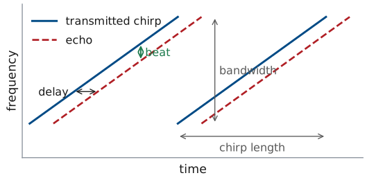
The transmitter sweeps \(B\) in \(T_s\), then starts again.
The echo is the same ramp, late by the round trip.
The gap between them, the beat, is constant.
An FMCW radar transmits continuously, and its frequency climbs linearly across a bandwidth \(B\) during each chirp of length \(T_s\). On the PHASER, in the Phaser app’s Range (Basic) preset, the chirp starts at 12.145 GHz and sweeps \(B = 500\) MHz in \(T_s = 1\) ms. The echo from a target at range \(R\) is a copy of the transmitted chirp delayed by the round trip,
which is 6.7 ns for every meter. The receiver compares the echo with the chirp that is still going out. Because both ramps climb at the same rate, the echo is always below the transmitted chirp by the same frequency, and that difference is the beat frequency \(f_b\). The figure exaggerates the delay so that it is visible: on the PHASER, a target at 3 m delays the echo by 20 ns, 0.002% of a 1 ms chirp.
The Beat Frequency
The transmitted frequency rises at the chirp slope \(B/T_s\), which for the PHASER is \(500\ \text{MHz}/1\ \text{ms} = 0.5\ \text{MHz}\) per microsecond. In the delay \(\tau\) the chirp climbs \(\tau B/T_s\), so the beat frequency is
The beat is proportional to range, so the radar reads range by measuring a frequency. A target at 1 m gives 3.33 kHz, and one at 3 m gives 10.0 kHz. These frequencies are low enough for the Pluto to sample directly, even though the chirp itself spans 500 MHz: comparing the echo with the outgoing chirp removes the sweep and leaves only the small difference that carries the range. ADI’s FMCW lab calls this stretch processing.
The kHz per meter depends on both waveform settings. Halving the bandwidth to 250 MHz halves it, to 1.67 kHz per meter, and halving the chirp length to 0.5 ms doubles it, to 6.67 kHz per meter. As the next frames show, only the bandwidth changes the resolution.
FMCW Explorer
The left panel is the beat signal over one chirp, with the 0 m frequency removed, and the right panel is its range spectrum, the FFT of those samples with the frequency axis converted to range. Move the target and count the cycles: every meter adds \(2B/c = 3.33\) cycles a chirp at 500 MHz. Halve the bandwidth or double the chirp length and watch the beat per meter halve; halve the chirp length and watch it double. Turn on the second target and bring it in toward the first until the two peaks merge; the green bar is \(c/2B\). Then set the second target 20 to 40 dB weaker and switch between the rectangular and Hann windows.
Range Resolution
Two targets separate when their beats differ by one cycle a chirp.
The chirp length cancels: only \(B\) sets the resolution.
The radar sees each target’s beat for one chirp, \(T_s\), and an FFT over a record of length \(T_s\) separates two tones only if they differ by at least \(1/T_s\). Over one chirp, that is a difference of one cycle. Converting that frequency step to range with the beat per meter gives
which is the result of Lesson 26. At 500 MHz it is 0.30 m. A longer chirp makes the beat per meter smaller but lets the FFT resolve finer frequency steps in the same proportion, so \(T_s\) cancels. Halving the bandwidth to 250 MHz doubles the resolution cell to 0.60 m; halving the chirp length to 0.5 ms leaves it at 0.30 m.
The number of beat cycles in one chirp is \(f_bT_s = 2RB/c\), which does not depend on \(T_s\) either. Two plates 0.30 m apart differ by exactly one cycle a chirp at 500 MHz; closer than that, their beats stay within one cycle of each other for the whole chirp and the FFT returns one peak.
The Range FFT
The app keeps 540 samples of each chirp, and one FFT turns them into a range profile.
Each FFT bin is 1.11 kHz, one 0.33 m range cell.
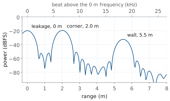
The PHASER’s Pluto samples the beat at \(f_s = 0.6\) MSPS, so one 1 ms chirp yields 600 complex samples. The app discards the first 0.1 ms of each chirp, while the frequency ramp settles, and keeps \(N = 540\). The FFT of those samples is the range profile: each bin is a frequency, and the beat-per-meter relation converts it to a range,
where \(f_0\) is the 0 m frequency of the next frame. The bins are \(f_s/N = 1.11\) kHz apart, which is 0.33 m, one resolution cell. That is a little more than the 0.30 m of the resolution frame because the 0.9 ms of each chirp the app keeps sweeps 450 MHz, not 500, and \(c/(2 \cdot 450\ \text{MHz}) = 0.33\) m. Padding the record with zeros before the FFT, to 4096 points or more, draws the same spectrum on a finer grid and makes the peaks easier to read, but it does not resolve anything new.
The figure is one chirp from the lab’s recorded data: a 10 cm corner reflector at 2.0 m, the transmit antenna’s direct path into the array at 0 m, and the far wall at 5.5 m. The top axis shows the same profile as beat frequency above \(f_0\), at 3.33 kHz per meter.
The FFT also integrates. The 540 samples of a steady tone add in phase while the noise adds in power, so the tone rises \(10\log_{10}540 = 27.3\) dB above the noise per sample, as Lesson 27 described. Seen another way, each bin collects noise from only 1.11 kHz. That is the narrowing Lesson 25 described: the corner at 3 m, 31.1 dB above the noise in 1 MHz, stands
above it in one bin.
The 0 m Frequency
The kit offsets the outgoing chirp by about 100 kHz, so a 0 m echo lands at \(f_0 \approx 100\) kHz.
Each kit’s \(f_0\) differs; Calibrate… reads it from a plate against the array.
The leakage spike always sits at \(f_0\).
The PHASER does not put a 0 m echo at zero frequency. The Pluto transmits its tone offset by signal_freq in ADI’s scripts, about 100 kHz, from the frequency the receiver compares the echo with, so every beat lands about 100 kHz above zero. That keeps the targets clear of zero frequency, where the receiver’s own offset and low-frequency noise sit. The offset is not exactly 100 kHz on every kit, and the cables and the board add a little delay of their own, so each kit has its own 0 m frequency \(f_0\), and the range equation measures beats from it.
The calibration is simple. Hold a flat metal plate against the array face, read the frequency of the peak, and record it as \(f_0\); ADI’s lab expects a value such as 99 or 103 kHz. With the plate gone, a peak stays at \(f_0\): it is the transmit antenna’s direct path into the array, the leakage, and it marks 0 m on every capture you take. A kit whose \(f_0\) is off by 1 kHz reports every range 0.30 m long or short.
Maximum Range from the Sample Rate
Halving \(B\) to 250 MHz doubles it to 120 m.
Halving \(T_s\) to 0.5 ms halves it, unless \(f_s\) rises too.
The Pluto samples complex data at \(f_s\), so it can represent beat frequencies up to \(f_s/2 = 300\) kHz. A target far enough away to put its beat above that limit aliases: it reappears at a wrong frequency, and the range profile shows it at a wrong range. With the 0 m frequency at 100 kHz, the beats above it have 200 kHz of room, so the farthest range the profile reports is
This limit comes from the sample rate, not from the transmit power; Lesson 25 put the detection range of a 10 cm corner near 8.5 m in a 1 MHz bandwidth, and farther out in the 1.11 kHz of one bin. A slower slope reaches farther: halving \(B\) halves the beat per meter and doubles \(R_\text{max}\) to 120 m, but it also doubles the resolution cell. A steeper slope reaches less far at the same sample rate, so the app’s Range (Fast) preset, 500 MHz in 0.5 ms, also samples at 5 MSPS: its 6.67 kHz per meter then reaches \((2.5\ \text{MHz} - 100\ \text{kHz})/(6.67\ \text{kHz/m}) = 360\) m. The lab measures both changes.
Windowing the Chirp
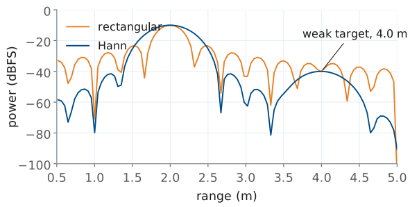
Rectangular: sidelobes at −13 dB hide weak targets.
Hann lowers the sidelobes to −31 dB but widens the main lobe 1.6 times and loses 1.8 dB of SNR.
An FFT of one chirp treats the record as if it started and stopped abruptly, which gives each tone a \(\sin x/x\) response with sidelobes 13 dB below the peak, falling slowly. A strong target’s sidelobes then cover the bins around it, and a weak target nearby disappears under them. In the figure the second target, 30 dB weaker and 2.0 m beyond the first, is invisible with the rectangular window.
Multiplying the samples by a window that tapers smoothly to zero at both ends of the chirp lowers the sidelobes. The Hann window,
puts the first sidelobe at −31 dB and the rest falling fast, and the weak target appears. This is the amplitude taper of Lesson 22 applied in time instead of across the array, with the same consequences: the main lobe widens, from a 3 dB width of 0.89 bins to 1.44 bins, so two equal targets one cell apart may merge, and the window discards some signal energy, a 1.8 dB loss in SNR. We use Hann by default; the rectangular window is the choice only when two equal targets must be split at the edge of the resolution.
The Range Waterfall
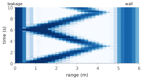
Each row is one range profile; time runs up.
Fixed objects draw vertical lines; a walker draws a zigzag.
The slope of the trace is the walker’s speed.
One range profile is a snapshot. Stacking the profiles of successive chirps, one row per chirp and darker for a stronger echo, gives the range waterfall: range across, time up. A fixed object, the leakage at 0 m or the wall at 5.5 m, keeps the same range in every row and draws a vertical line. A person walking from 1 m out to 4 m and back draws a zigzag, and the slope of each leg is the walking speed: a 3 m leg in 3 s gives 1 m/s.
The waterfall records range against time and nothing else. Its rows here are 50 ms apart, one profile each time the display updates, and over 50 ms a walker’s carrier phase changes by many cycles, so successive rows say nothing about the walker’s velocity except through the range they show. Lesson 29 takes chirps a fixed 0.5 ms apart and reads the velocity from that phase.
The Provided Range FFT
def range_fft(cap, window="hann",
              n_fft=None):
    iq = cap["iq"]
    w = _window(window, iq.shape[1])
    X = np.fft.fft(iq * w, n_fft or
                   iq.shape[1], axis=1)
    return X / w.sum()
The course provides
radar_lab.py, complete.Each lab’s notebook changes a line or two of it.
The four labs that follow share one Python module, radar_lab.py, and one capture format. The course provides the module complete: you run it from a notebook, one for each lab, and each lab’s tasks change a parameter or a line or two, never a whole function. The excerpt is the function this lesson describes: it windows every chirp, takes the FFT along each one, and divides by the sum of the window, so that a tone of amplitude 1 reads 0 dBFS whatever the window. n_fft larger than the samples in a chirp zero-pads it. The result has one row per chirp and one column per range bin.
A capture is an .npz file holding iq, the complex beat samples of the summed array with one chirp a row, shape n_chirps × n_samples; optionally iq_ch, the same samples from the array’s two halves, shape 2 × n_chirps × n_samples, which Lesson 31 uses to measure angle; the sample rate fs; the carrier fc; the bandwidth B; the chirp length T_ramp, the lesson’s \(T_s\); the time PRI from one chirp to the next; and f0, the 0 m frequency from your calibration, or the 100 kHz IF tone in a capture saved before it. The number of chirps is not fixed: 32 in an L28 range capture, 256 in the L29 burst, and thousands in a record of several seconds. The range of each bin comes from range_axis, the range equation of the range FFT frame with k the meters per hertz of beat:
def range_axis(cap, n_fft=None):
    n = n_fft or cap["iq"].shape[1]
    f = np.fft.fftfreq(n, 1 / cap["fs"])
    k = C * cap["T_ramp"] / (2 * cap["B"])
    return (f - cap["f0"]) * k
The bins come out in the order np.fft.fft returns them, and the bins below \(f_0\) come out as negative ranges. Two more L28 functions build on range_fft: range_profile(cap, chirp=0, window="hann") returns one chirp’s ranges at or beyond 0 m and its power in dB, (r, p_db), and waterfall(cap) returns (r, t, w_db), one row per chirp. Lesson 29 uses range_doppler and mti, Lesson 30 uses cfar_2d, and Lesson 31 uses the spectrogram, a classifier, and a tracker, all in the same module. The L28 notebook is L28_range.ipynb.
L28 Lab: FMCW Range
Calibrate \(f_0\), then put a plate at 1, 2, and 3 m: measure the kHz per meter.
Predict, then measure, the beat with a 0.5 ms chirp and at 250 MHz.
Read the waterfall; run the notebook’s three tasks.
The L28 Lab measures everything this lesson derived, on your own kit: the 0 m frequency, the beat per meter, how the chirp length and the bandwidth change it, and the range waterfall. The Phaser app does the live work: the 0 m calibration, the range profile, the waterfall, and saving captures. The course’s notebook does the rest. It reads the frequency of each peak from the captures you saved, which the app does not display, and it runs the provided range FFT on them, with one line changed for each of three tasks. You work the lab on your own, outside class, and turn in one packet in three parts: Part 1, Pre-Lab, the predictions, before you go to the bench; Part 2, Measurements, from your own kit; and Part 3, Writeup, after it. I check the packet and return it with feedback. It is the first piece of scaffolding for your final report, and it is not the report.
The procedure is ADI’s FMCW lab run on the app’s Range (Basic) preset: a 12.145 GHz carrier, 500 MHz in 1 ms, 0.6 MSPS, and \(c = 3.00\times 10^8\) m/s. The radar setup page describes the transmit path.
Pre-Lab Predictions
Waveform |
kHz per meter |
\(\Delta R\) |
\(R_\text{max}\) |
|---|---|---|---|
Range (Basic): 500 MHz, 1 ms |
3.33 |
0.30 m |
60 m |
Range (Fast): 500 MHz, 0.5 ms |
6.67 |
0.30 m |
360 m |
250 MHz, 1 ms (recorded) |
1.67 |
0.60 m |
120 m |
The table is the core of Part 1. Every number in it follows from the beat-frequency, resolution, and reach frames, with \(f_0 = 100\) kHz, \(f_s = 0.6\) MSPS for 1 ms chirps, and 5 MSPS for Range (Fast). The app has no bandwidth control, so the 250 MHz row comes from the course’s recorded capture. The bench checks each column. The beat per meter is the slope of the line through your 1, 2, and 3 m readings. The resolution shows as the width of the peak: at 250 MHz the peak from the same plate is twice as wide in range, and at 0.5 ms it is as wide as at 1 ms. The reach is not something the lab can walk out to, but the range axis shows where it ends.
The 0.5 ms chirp also changes the height of the peak. A bin’s noise bandwidth is the inverse of the record length, so halving the chirp doubles the noise in each bin while the echo’s power stays the same, and the plate’s peak stands about 3 dB lower above the noise floor.
Bench Rules
Transmit antenna on OUT2, before you power the kit.
Stand clear of the beam while you measure a static target.
Use a flat metal plate, square to the array, at array height.
A static measurement requires that nothing else in the beam moves. Your own body is a larger reflector than a small plate, so step behind the kit or well to one side while you read a static range; otherwise your echo adds a moving peak near the target’s and the profile you save is not the one you meant to save. Keep the beam’s path clear of walls and furniture for at least 4 m if you can, and expect the far wall to show up as a peak of its own.
Any flat metal plate about 20 cm on a side works, and so does aluminum foil glued smoothly to cardboard. A plate reflects strongly only when it faces the array squarely, so turn it slowly until its peak is highest before you save. A trihedral folded from three foil-covered cardboard squares is more forgiving of its angle. I have only one or two commercial corner reflectors; no step needs one, and if one is free, Part 2 has an optional reading for it. Measure range from the array face to the plate’s front with a tape measure.
Results
Your captures, and the file name of each in the packet.
Your \(f_0\) and your measured kHz per meter.
A screenshot of your walk’s waterfall, and the notebook.
Keep your captures, the notebook, and radar_lab.py together in your Module 4 folder. For the final report, keep three results from this lab: the beat per meter you measured against the 3.33 kHz the lesson predicts, the resolution you saw at 500 and 250 MHz, and a waterfall you can explain line by line. The report asks you to explain how a chirp becomes a range measurement and the resolution you measured, in your own words; the packet’s tables are the evidence for it, not the explanation.
Equipment and Setup
You need:
the ADALM-PHASER kit with its Raspberry Pi and Pluto attached, and its transmit antenna;
a flat metal plate about 20 cm on a side, or foil glued to cardboard;
a tape measure and about 4 m of clear floor in front of the kit;
your laptop, on the kit’s network for the Phaser app, and set up for the notebook as the Notebook Setup frame describes.
The radar half of the Phaser app is on port 8081 of your kit, beside the beamforming dashboard on 8080. Its FMCW panel is the FMCW section of the settings column, and each range view is a tab above the plot.
With the kit powered off, connect the transmit antenna to OUT2.
Power the kit, wait for the Pi to boot, and browse to
http://phaser-NN.local:8081, with your kit’s number.Choose the FMCW mode tab at the top of the settings column and open the FMCW section. Its status line should read FMCW ready. If it reads FMCW limited, hover over it for the reason and tell me: the kit has no chirp sync, so its chirps are not the preset’s, and the recorded data stand in for your Tables B and C.
Set Preset to Range (Basic), leave Range Max (m) empty, and press Start. The Range tab shows one range profile per display update, and the readouts under the plot give Peak Range, the strongest return, and Frame Rate.
Save Capture downloads the course’s capture format to your laptop as
phaser_range_<date>-<time>.npz: 32 chirps of 540 samples. Move each file into your Module 4 folder as you save it, rename it if you like, and write its name in the packet.
No Hardware?
Note
If your kit will not run, every procedure works in the app’s simulator, in a browser with no kit and no install, on the course’s recorded data. Open livethisdream.github.io/phaser/radar, choose the FMCW mode tab, and follow the procedures as written. Two controls replace the bench:
Load Recording, in the FMCW section, plays one of the course’s captures through every view as if it were live: Calibrate, the Range and Range Waterfall tabs, and the readouts. Stop ends it. The recording sets the waveform, so the app grays out Preset while it plays.
Scene, in the simulator only, picks a live simulated room. Corners puts corner reflectors at 1, 2, and 3 m, and Walker walks from 1 m out to 4 m and back.
The recorded captures are in the lab’s bundle, L28_lab.zip, with the notebook: a simulation of the PHASER at Range (Basic), with a kit whose 0 m frequency is 101.4 kHz, a 10 cm corner reflector standing in for the plate, and tape readings a few centimeters off, as a real bench’s are. Each procedure names the file for each step, and the notebook reads every one. Mark in your packet which rows come from the recorded data.
Procedure A: Calibrate the 0 m Frequency
Clear the bench in front of the kit and run Range (Basic). If 0 m Beat (kHz) holds a value from an earlier session, open Calibrate… and press Reset to clear it.
With the bench clear, open Calibrate… again if you closed it. The Strongest return is the leakage from the transmit antenna into the array, a few tenths of a meter out. Its frequency is New 0 m beat: record it in Table A as the leakage, then press Cancel. Save a capture of the clear bench.
Hold the plate flat against the array face, covering the patches, and save a capture.
Open Calibrate… again, wait for Strongest return to settle, record New 0 m beat as the app’s \(f_0\) in Table A, and press Calibrate. 0 m Beat (kHz) now holds it, the range axis reads 0 m there, and every capture you save from now on carries it as its
f0.
The range axis starts at 0 m, so a kit whose \(f_0\) is below the 100 kHz IF tone puts the plate at a negative range, off the plot, and Strongest return finds something else. If the plate’s peak is missing, type 95 in 0 m Beat (kHz) and open Calibrate… again. The app reads frequencies to the nearest FFT bin, 1.11 kHz, so its \(f_0\) can be off by up to half a bin, about 0.2 m of range. The notebook’s peak readout reads the same two captures to 0.01 kHz; record both, and use the notebook’s value in task (c). No kit: load L28_clear.npz for step 2 and L28_cal_0m.npz for steps 3 and 4. Both carry the IF tone as their f0, as yours do, because they come from before the calibration.
Procedure B: Static Ranges
Stand the plate at 1.00 m from the array face, at array height, facing the array squarely. Step out of the beam.
On the Range tab, turn the plate slowly until its peak is highest. Hover over the peak, record its range in Table B with the tape-measure range, and save a capture.
Repeat at 2.00 m and 3.00 m. At each range, check that the plate’s peak moved out by about 1 m before you save; a peak that did not move is the leakage or the wall. Peak Range shows the strongest return, which at 3 m can be the leakage near 0 m, so read the plate’s peak by hovering over it.
If one of the course’s corner reflectors is free, put it at 3.00 m instead of the plate and save one more capture for the optional row of Table B.
The app’s range axis comes from the beat per meter it assumes, so the range it shows cannot test that number; the frequencies the notebook reads from your three captures can, and they fill the rest of Table B. No kit: load L28_corner_1m.npz, L28_corner_2m.npz, and L28_corner_3m.npz, or set Scene to Corners for a live look.
Procedure C: Chirp Length and Bandwidth
Write your Part 1 predictions in Table C before you change anything.
The reference row is your Procedure B capture at 2.00 m, at Range (Basic).
Leave the plate at 2.00 m and set Preset to Range (Fast), 500 MHz in 0.5 ms at 5 MSPS. The plate should still read about 2 m, because the app rescales its range axis to the new chirp. Save a capture.
The app has no bandwidth setting, so everyone uses the course’s 250 MHz capture: load
L28_corner_2m_B250.npzwith Load Recording and compare the width of the plate’s peak with your own 500 MHz peak. Press Stop when you are done.Return Preset to Range (Basic).
The notebook’s peak readout gives each row’s peak frequency, its width 3 dB down, and its height above the noise floor. No kit: load L28_corner_2m_fast.npz for step 2.
Procedure D: Read the Waterfall
Open the Range Waterfall tab. Under Display, set Waterfall Depth to 200, and in the FMCW section set Range Max (m) to 6. Time runs down the plot in display updates, frames ago.
Stand 1 m in front of the kit, facing it. Walk slowly straight out to about 4 m and back, about one step a second, twice. Then hold a hand 0.5 m from the array and move it toward and away from the array.
If the fixed lines crowd your trace, lower Color Span (dB) until they are faint and your trace is still bright.
Take a screenshot of the waterfall with your two walks on it. Hover over the trace to record in Table D the nearest and farthest ranges it reached and the number of frames one leg took, and record the Frame Rate readout.
A saved capture holds only 32 chirps, a fraction of a second, so the waterfall plot in the notebook comes from the course’s 10 s walk, L28_walker.npz. No kit: set Scene to Walker and press Start, or load L28_walker.npz; both walk from 1 m to 4 m and back at 1 m/s.
Notebook Setup
The notebook runs on your own laptop, with Python 3 and four packages: numpy, scipy, matplotlib, and Jupyter. You need nothing else, and once they are installed the notebook runs without a network connection.
Install Python 3.10 or newer from python.org if your laptop does not have it. Then, in a terminal, install the four packages in one line:
python -m pip install numpy scipy matplotlib jupyterlab
Make a folder for the Module 4 labs, such as
ece444-radar, download the lab’s bundle,L28_lab.zip, and unzip it into the folder. It holdsL28_range.ipynb,radar_lab.py, every recorded capture the procedures name, and a README that lists them.Move your own captures into the same folder.
In a terminal, change to the folder and start Jupyter with
jupyter lab. OpenL28_range.ipynband run its first cell: it prints the capture’s chirps, samples, bandwidth, chirp length, sample rate, and \(f_0\). If it reports thatradar_labis missing, the module is not in the same folder as the notebook.
Keep this folder for the whole module. Each later lab adds its own bundle to it, and they all use the same radar_lab.py.
Procedure E: Run the Notebook
Do this part after the bench, from your saved captures, in about 30 to 45 minutes.
Open
L28_range.ipynb, setCAPTUREin the first code cell to your 2 m capture, and run the cells from the top.Peak readout: set
NAMEto each capture Tables A to C name, one at a time, and record the peak frequencies, widths, and heights it prints.Task (a): run the range-profile cell with
WINDOW = "hann", then change that one line toWINDOW = Noneand run it again. Record the peak, the strongest sidelobe, and the floor near 10 m for each window in Table E.Task (b): in the two-corner cell, the only cell with an
N_FFTline, run it withN_FFT = None, then change that line toN_FFT = 4096. Record how many peaks it finds and the width 3 dB down each time.Task (c): set
F0to your Table A value from the notebook and replaceR = Nonewith the range of the peak, fromf_peak,F0, and the capture’sBandT_ramp. RecordRin Table E and compare it with the tape.Run the waterfall cell for the waterfall plot.
Save the notebook with its edits and plots, and upload the
.ipynbwith the packet.
Each cell’s markdown states the result to check against, for the recorded data. Anything you do beyond the three tasks belongs in your report’s Extra Effort.
Lab Packet
Summary
Idea |
What it is |
Number to remember |
|---|---|---|
Beat frequency |
\(f_b = 2RB/(cT_s)\), the echo compared with the chirp still going out |
3.33 kHz per meter at 500 MHz, 1 ms |
Beat cycles a chirp |
\(f_bT_s = 2RB/c\) |
3.33 cycles per meter at 500 MHz |
Range resolution |
one FFT bin, \(1/T_s\), is \(c/2B\) in range |
0.30 m at 500 MHz, 0.60 m at 250 MHz |
Range from frequency |
\(R = cT_s(f - f_0)/2B\) |
bins 1.11 kHz, 0.33 m, apart for the 540 samples the app keeps |
0 m frequency |
\(f_0\), calibrated per kit; the leakage sits there |
about 100 kHz |
Reach |
\(R_\text{max} = cT_s(f_s/2 - f_0)/2B\) |
60 m at 0.6 MSPS, 1 ms |
FFT integration |
540 samples add in phase |
27.3 dB, a 1.11 kHz noise bandwidth |
Hann window |
sidelobes −31 dB instead of −13 dB |
main lobe 1.6 times wider, 1.8 dB SNR loss |
Waterfall |
range profiles stacked in time |
slope of a trace is the speed |
Looking Ahead
L29 stacks 256 chirps, 0.5 ms apart, and reads velocity from their phase.
The
range_fftyou ran here is the first FFT of its range-Doppler map.
This lesson used one chirp at a time and discarded its phase, which Lesson 29 keeps. A burst of 256 chirps, each 300 µs long and repeated every 0.5 ms, gives each target a phase that advances from chirp to chirp at its Doppler frequency, and a second FFT across the chirps reads that frequency as a velocity, with the resolution of Lesson 26,
The first FFT of that map is the range FFT you ran here, applied to every chirp of the burst. Moving target indication, in the same lesson, removes the fixed lines of the waterfall, the leakage and the wall, so that only what moves remains.