A radar sends a known signal and listens for the copy a target reflects. The copy differs from what was sent in four ways, and each difference is a measurement. It arrives late, by the time the wave needs to reach the target and come back, which gives range. It arrives shifted in frequency if the target is moving toward or away from the radar, which gives radial velocity. It arrives with a phase ramp across the array that depends on its direction, which Module 3 turned into an angle: the beam sweep of L19 reads it with one channel, and the monopulse comparison of the two subarray channels in the L24 Lab reads it in a single snapshot. And it arrives weaker by an amount the radar equation of L25 predicts, so the received power says something about the target’s cross section.

This lesson covers the first two. Module 3 covered angle and L25 covered power, and L27 combines them with noise to decide whether an echo is there at all.

The transmitted wave travels at \(c\) out to the target, reflects, and travels the same distance back, so the echo arrives a time \(\tau = 2R/c\) after the transmission. Turned around, a measured delay gives the range,

The factor of 2 comes from the round trip: range is half the distance the wave covered. With \(c = 3.00\times 10^8\ \text{m/s}\), every meter of range adds \(2/c = 6.67\ \text{ns}\) of delay. A target across the lab, 3 m from the kit, returns its echo after 20 ns, which is far too short to time directly with the Pluto’s sample clock; L28 shows how the FMCW waveform converts that delay into a frequency the Pluto can measure. An aircraft 6 km out returns its echo after \(40\ \mu\text{s}\), which a pulsed radar times directly.

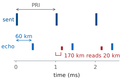
A pulsed radar does not send one pulse; it sends a train of them, one every pulse repetition interval \(T_\text{PRI}\), at a pulse repetition frequency \(\text{PRF} = 1/T_\text{PRI}\). The receiver times each echo from the most recent pulse, because it has no way to tell which pulse an echo belongs to. That works as long as every echo comes back before the next pulse leaves, which holds for every target closer than

the unambiguous range. At a PRF of 1 kHz it is 150 km. A target farther out still reflects, but its echo arrives after the next pulse has gone out, and the receiver times it from that pulse. In the figure a target at 170 km returns its echo 1.133 ms after its pulse, which is 0.133 ms after the next one, so the radar reports it at \(170 - 150 = 20\ \text{km}\). Radars remove this ambiguity by changing the PRF from one burst to the next: a true range stays put, and a folded one moves.

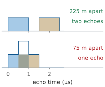
Resolution is the ability to report two targets as two. Suppose two targets sit \(\Delta R\) apart in range, and the radar sends a pulse of length \(\tau_p\). Their echoes are each \(\tau_p\) long and start \(2\Delta R/c\) apart. When that gap is longer than the pulse, the receiver sees two echoes with a quiet interval between them; when it is shorter, the echoes overlap, and the receiver sees a single longer echo it cannot split. The boundary is \(2\Delta R/c = \tau_p\), so the range resolution is

A \(1\ \mu\text{s}\) pulse resolves targets 150 m apart. In the figure the targets 225 m apart give two echoes, and the targets 75 m apart give one. Where two echoes overlap they add as phasors, so the overlap is stronger or weaker than either echo depending on their relative phase; the figure shows them in phase.

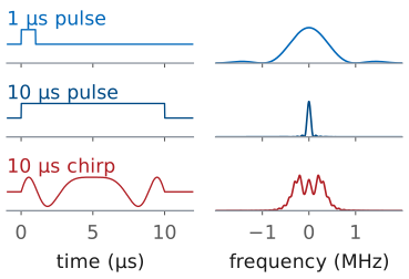
A short pulse resolves well but carries little energy, since energy is power times duration, and every transmitter has a peak-power limit. Detection, L27’s subject, needs energy; resolution needs a short pulse. A short pulse resolves well because of its bandwidth. A pulse’s spectrum is the Fourier transform of its envelope, and a rectangle of length \(\tau_p\) transforms to a sinc whose main lobe is about \(1/\tau_p\) wide. That is the transform L15 applies to a uniform aperture, where a length \(L\) gives a beam about \(\lambda/L\) wide: the shorter the pulse, the wider its spectrum. A pulse of length \(\tau_p\) therefore occupies a bandwidth of about \(B \approx 1/\tau_p\), and the resolution can be written

This form is the general one, because what separates two echoes is the bandwidth of the waveform, not its length. A chirp, a pulse whose frequency sweeps across \(B\) during a long transmission, has the bandwidth of a short pulse and the energy of a long one. Comparing the echo with the outgoing chirp turns each delay into a different frequency, so two echoes \(1/B\) apart in delay separate in frequency, and the radar recovers the resolution \(c/2B\). L28 derives this as stretch processing; a pulsed radar does the equivalent with pulse compression. ADI’s FMCW lab sweeps the PHASER’s transmitter across 500 MHz, which gives \(\Delta R = 0.30\ \text{m}\): two corner reflectors on the bench must be more than 30 cm apart in range to appear as two. L28 derives the FMCW version of this result.

The figure puts the three waveforms side by side. The \(1\ \mu\text{s}\) pulse spreads over about 1 MHz, and the \(10\ \mu\text{s}\) pulse, ten times longer, over about a tenth of that. The \(10\ \mu\text{s}\) chirp sweeps 1 MHz, so it lasts as long as the long pulse and carries its energy, while its spectrum is as wide as the short pulse’s.

The echo’s phase records the round trip. A wave that travels \(2R\) picks up a phase relative to the transmitted signal of

If the target moves, \(R\) changes with time and so does that phase, and a phase that changes steadily with time is a frequency. Differentiating gives the Doppler shift

where \(v_r = -dR/dt\) is the rate at which the range is closing. The 2 is the same factor as in \(R = c\tau/2\): the path changes twice as fast as the range. At a 10 GHz carrier, \(\lambda = 3.0\ \text{cm}\) and each meter per second of closing speed shifts the echo by 66.7 Hz.

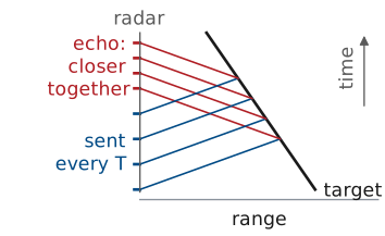
The figure draws the same result as crests in time and range, with the target’s speed exaggerated so the effect is visible. Each crest leaves the radar a time \(T\) after the one before, meets the target a little closer in, and so has a shorter trip back. The echoes arrive spaced \(T(c - v_r)/(c + v_r)\) apart, less than \(T\), which is a higher frequency; for \(v_r \ll c\) that is the \(2v_r/\lambda\) shift above.

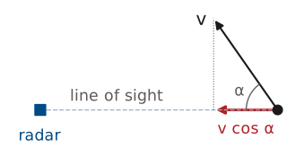
The course convention is the usual one: a target moving toward the radar has positive \(v_r\) and a positive Doppler shift. As the range shrinks, each wave crest has a shorter trip than the one before, so the crests arrive closer together and the echo’s frequency is higher than the transmitted one. A target moving away stretches the crest spacing and shifts the echo down.

Only motion along the line of sight changes the range. A target moving at speed \(v\) in a direction \(\alpha\) off the line of sight has

An aircraft at 200 m/s flying 60° off the line of sight closes at 100 m/s and shifts a 10 GHz echo by 6.67 kHz. One crossing the line of sight at \(\alpha = 90^\circ\) has no Doppler shift at all. A Doppler radar removes zero-Doppler returns, because the ground, the walls, and every other fixed reflector sit there (the clutter that L29’s MTI removes), so a target moving fast but tangentially is removed with them.

ADI’s CW radar lab (Analog Devices, “CW Radar with Phaser”) takes a car at 100 mph as its example. In meters per second that is 44.7 m/s, and

at 2.4 and 10 GHz. ADI quotes 716 and 2982 Hz; the difference is only the value of \(c\), which they take as \(2.998\times 10^8\) rather than the course’s \(3.00\times 10^8\ \text{m/s}\). A higher carrier gives a larger shift for the same speed, since \(f_D\) scales as \(1/\lambda\).

Both shifts are tiny next to the carrier. No receiver could measure a 10.000003 GHz echo directly against a 10 GHz reference with any accuracy, so a Doppler radar compares the echo with its own transmitted signal and keeps only the difference, which comes out at a few hundred or thousand hertz, where the Pluto digitizes it easily.

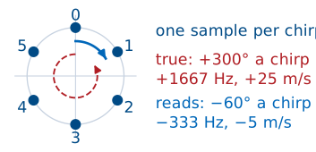
Range and Doppler have the same two limits. To tell two frequencies apart, the radar has to watch the echo long enough for them to drift a full cycle apart, so an observation of length \(T\) resolves frequencies \(1/T\) apart. Divided through by \(2/\lambda\), that is a velocity resolution

A pulsed radar sees the target only once per pulse, so it samples the Doppler phase at the PRF. Those samples are complex, so by the sampling theorem of L17 they cover a window one sampling rate wide, \(\pm\text{PRF}/2\). A faster target aliases into that window and reports the wrong speed, possibly the wrong sign. Setting the largest shift equal to the window edge gives the unambiguous velocity:

ADI’s range-Doppler lab (Analog Devices, “Range Doppler Radar Processing”) sends a burst of 256 chirps, 0.5 ms apart, near 10 GHz. The burst lasts \(T = 128\ \text{ms}\), so it resolves 7.8 Hz, or 0.12 m/s, and its unambiguous velocity is ±15 m/s. A person walking is well inside that window; a car on a highway is not. L29 builds the range-Doppler map from exactly this kind of burst.

The figure follows a car closing at 25 m/s through this burst. Its true shift is 1667 Hz, so the phase advances 300° from one chirp to the next. The samples alone cannot tell that from a step of −60°, which is −333 Hz, and the radar reports a target moving away at 5 m/s.

The PRF appears in both unambiguous limits, in the denominator of one and the numerator of the other. A low PRF leaves a long listening time between pulses, so the unambiguous range is long, but it samples the Doppler slowly, so the unambiguous velocity is small. A high PRF does the reverse. The product of the two does not depend on the PRF at all:

At 10 GHz that is \(1.1\times 10^6\ \text{m}^2/\text{s}\). A 1 kHz PRF gives 150 km of unambiguous range and only ±7.5 m/s of unambiguous velocity, about 17 mph, the speed of a fast bicycle. An airborne radar that must report both range and closing speed for fast aircraft cannot satisfy both limits with one PRF, so it switches among several and works out the true range and velocity from how the readings move, the same idea used against a folded range above.

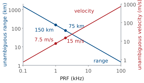
The figure plots both limits against PRF at 10 GHz. The range limit falls and the velocity limit rises at the same rate, so no PRF moves one without moving the other the opposite way.

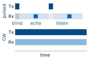
ADI’s radar setup page (Analog Devices, “Setup the Phaser for Radar”) divides radars into two families. A pulsed radar transmits a short, powerful pulse, switches its one antenna over to the receiver, and listens until the next pulse. It times echoes directly, reaches long ranges because its peak power is high, and cannot hear anything while it transmits: a target closer than \(c\tau_p/2\) returns its echo while the pulse is still going out.

A continuous-wave (CW) radar transmits and receives at the same time. Its transmitter never switches off, so it needs a separate transmit antenna, far enough from the receive antenna that the leakage between them does not overwhelm the echo. Its average power is modest, which suits short ranges, and it has no blind zone near the radar. That makes it the right choice for a radar on a lab bench. The PHASER is set up this way: the transmit antenna on OUT2 sits beside the eight-element receive array, at the same height.

The simplest CW radar sends a single unmodulated tone. Its echo is the same tone, delayed and shifted by \(f_D\). The shift is easy to measure: compare the echo with the transmitted tone and the difference is a sine wave at \(f_D\), whose frequency an FFT reads directly. The delay is not measurable at all. Every cycle of a pure tone looks like every other cycle, so there is no feature in the echo to time against the transmission. A CW radar therefore measures speed but not range, which is all a police speed radar requires.

The FFT of the CW echo is one spectrum for the whole beam. A car and a fence behind it both reflect; the fence sits at 0 Hz and the car at its \(f_D\), and two cars at the same speed fall in the same bin regardless of range. L28’s FMCW waveform restores the time mark: it sweeps the transmitted frequency in a ramp, so the frequency of the echo says when it was sent, and the delay becomes a measurable frequency difference.

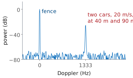
The figure is a simulated CW spectrum of that scene at 10 GHz. The fence is the strong line at 0 Hz. Two cars close at 20 m/s, one at 40 m and one at 90 m; their ranges change only each echo’s phase, so both land in the single line at 1333 Hz.

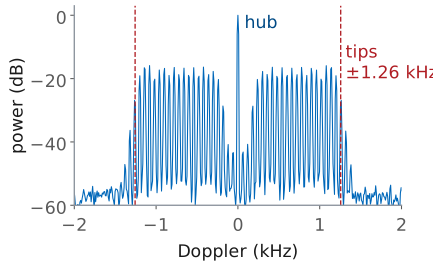
ADI’s CW lab points the PHASER at a variable-speed fan and shows its Doppler spectrum as a waterfall, successive spectra stacked in time. ADI’s script takes 65,536 samples at 0.6 MHz for each spectrum, 109 ms of echo, so by \(\Delta f = 1/T\) its bins are 9.2 Hz wide, or 0.14 m/s at 10 GHz.

A fan is a useful target because its body stays in place while its blades move. Seen edge-on, a point on a blade at radius \(\rho\) swings toward and away from the radar at up to \(\Omega\rho\), where \(\Omega\) is the rotation rate in radians per second. The tips move fastest: a 0.3 m fan at 1200 rpm has a tip speed and a peak Doppler shift of

The spectrum fills the band between, one return for each part of each blade, while the hub and the stand stay at 0 Hz. Speed the fan up and the band widens in proportion; the edge of the band measures the tip speed. Face the fan head-on and the blades move across the line of sight instead of along it, and the band collapses toward 0 Hz. The line spacing in the figure comes from the three blades passing 20 times a second, 60 Hz.

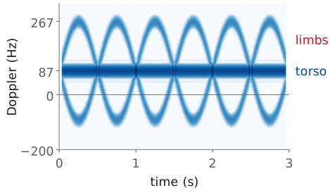
The fan is one case of a general effect. A target is rarely one rigid body moving at one speed. A walker’s torso approaches at a steady speed, while the arms and legs swing forward and back about it; a helicopter’s rotor spins on top of a fuselage; a drone’s propellers spin on a hovering frame. Each moving part adds a Doppler shift of its own on top of the body’s, and the extra shifts, called micro-Doppler, change in time with the motion.

A single spectrum blurs those changes together. A spectrogram, a run of short spectra plotted against time, shows them. The figure is a simulation of a walker approaching at 1.3 m/s at 10 GHz: the torso produces the steady line at 87 Hz, and two limbs swinging in opposite phase, once a second, trace sinusoids that reach 267 Hz (4.0 m/s) going forward and about −93 Hz going back. The spectrogram trades resolution for time: each column uses 64 ms of echo, so it resolves only about 16 Hz, by the same \(\Delta f = 1/T\).

A walker, a fan, a fidget spinner, and a waving hand each produce a distinct pattern. L31 turns those patterns into features, and the L31 Lab classifies those four targets from spectrograms recorded on your own kit.

Most of this lesson’s quantities come back in the labs. L27 adds noise and asks how reliably a radar decides that an echo is present. L28 sets up the PHASER’s FMCW mode, where the chirp’s 500 MHz sets the 0.30 m range resolution and the delay of each echo appears as a beat frequency; the L28 Lab measures it on corner reflectors. L29 sends a burst of chirps and forms the range-Doppler map, with the velocity resolution and the unambiguous velocity defined here as its axes. L31 returns to micro-Doppler and classifies targets from their spectrograms.