L24 Lab — Null Steering#
Null Steering
A computed notch, a structural null, an adaptive null, and the monopulse pair, measured on your own kit.
L24 Lab · Antennas, Phased Arrays, and Radar Systems · Dr. Neil Rogers
Printing
To print the slides, switch to present mode and print: one slide a sheet, with room for notes. Print from read mode for the whole lesson.
Learning Objectives
- I can calculate null-steering weights and implement pattern nulls on the ADALM-PHASER.
Lesson 24 ended with a weight vector on paper: eight complex numbers that hold the beam on the target and put a pattern null on the interferer. Today we load those numbers into the array and measure what the hardware gives back. The lab runs four procedures, in increasing order of how much the array does for itself: a static notch you compute yourself (A), a boresight null that comes from subtracting the two digital channels (B), an adaptive beamformer that finds its own null from the received data (C), and the same difference beam put to a different use, measuring a target’s angle from a single look (D). That last one is where Module 4 begins.
What Lesson 24 Predicts
Element |
Gain (%) |
Phase (deg) |
|---|---|---|
1 |
74 |
−12.0 |
2 |
65 |
+3.5 |
3 |
82 |
+13.0 |
4 |
100 |
+6.0 |
5 |
100 |
−6.0 |
6 |
82 |
−13.0 |
7 |
65 |
−3.5 |
8 |
74 |
+12.0 |
The main lobe drops about 2 dB.
The weight-subtraction rule of Lesson 24 holds the beam at broadside and nulls an interferer at \(\theta_1 = +22.5^\circ\):
The table converts the weights to what the GUI accepts: element gain as a percentage of the largest, \(100\vert w_n\vert/\max\vert w\vert\), and phase offset as \(\angle w_n\), entered with its sign. It is worked at 10.443 GHz, the frequency Find HB100 reported for phaser-00, one of the course kits. Part 1 of the packet has you compute the same table at your own kit’s frequency; at the nominal 10.525 GHz the outer gains read 75 % and the phases of elements 2 and 7 read ±3.1°, so the table moves only slightly from kit to kit.
The predictions assume the Element Gains slider is linear in voltage, which it is on current Phaser software. On phaser-00 the main lobe dropped 2.5 dB against the predicted 2.0.
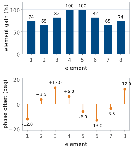
The gains are symmetric about the array center and the phases are antisymmetric, the conjugate mirror pairs of Lesson 24’s weight circle. Neither column nulls anything on its own; only the eight weights together do.
Why the Notch Goes Deep
One-step channel errors allow a notch about 48 dB below the uniform peak.
phaser-00: 46 to 50 dB open, 22 to 24 dB cramped.
A shallow notch points to the bench first: reflections, calibration, or a sign.
Lesson 24 estimated the depth that small, independent channel errors allow, about 48 dB below the uniform peak, and the 2026-10-23 dry run on phaser-00 reached 46 to 50 dB. Rounding the weights to the ADAR1000’s 2.8125° and 1 % steps does not set that limit: the rounded table keeps its mirror symmetry, so its null survives and moves only a fraction of a degree. On a freshly calibrated kit the notch landed at +21.7°. In a cramped space on 2026-10-25 the same table bottomed out 22 to 24 dB down, and so did the difference null of the next frame: the HB100’s own tone was still there in the null, so a reflection arriving from another direction, about 22 dB below the direct path, was filling both.
When a notch reads much shallower than 40 dB, look at the bench before the arithmetic. A wall or a person beside the kit fills it, a stale calibration fills it, and a sign error on the phase column moves it to −22.5°, where it is easy to miss.
The Difference Beam
Beam 1 Phase \(= 180^\circ\) subtracts the two subarray channels.
Boresight becomes a null, with peaks near ±11°.
A computed null sits where we solved for it; a structural null sits where the two subarrays cancel.
There is a second null on this board that needs no computation at all. Each ADAR1000 sums its four elements into one RF channel, so the PHASER hands the Pluto two digital subarray channels, one for elements 1–4 and one for elements 5–8. Adding them is the ordinary sum beam. Subtracting them, by setting Beam 1 Phase to 180°, cancels the two halves wherever they arrive in phase, which is boresight. The result is a null there with twin peaks near ±11°: the monopulse difference beam, which Procedure D and Module 4 use for angle measurement. On phaser-00 it measured −41.5 dB on an open bench and −22 dB in a cramped one, centered on boresight, with the peaks at ±12.0°. It needs no arithmetic, so its depth is a direct reading of what the room lets through.
The +22.5° notch exists because we solved for eight weights, and it moves only when we solve again. The boresight null exists because the two subarrays are identical, and it stays at boresight no matter what the signal does.
MVDR
Minimum output power, with unit gain in the look direction \(\mathbf{s}\).
\(\mathbf{R}\) is estimated from the data, so nobody supplies the interferer’s angle.
Procedures A and B both needed something known in advance: the interferer’s angle in A, the array’s symmetry in B. The MVDR (minimum-variance distortionless-response) beamformer needs neither. It estimates the covariance of what the two channels receive over \(K\) snapshots,
and solves for the weights that minimize total output power while holding unit gain in the look direction \(\mathbf{s}\). Whatever is loud and is not in the look direction is suppressed, and the beamformer never has to be told where it is.
Unit gain means the two MVDR weights sum to 1 in the look direction, where Manual’s two weights of 1 sum to 2. The Phaser multiplies the MVDR output by 2, the number of channels, so a target in the look direction reads the same level under either mode and the two are compared on one scale.
Two Limits of Two Channels
Near ±30° the subarray pattern already puts the interferer 20 dB down.
There the two channels cannot tell it from boresight, so MVDR’s one null hits the target.
Diagonal loading limits that loss; Procedure C runs at +20°.
Both limits belong to the architecture rather than to the algorithm. A four-element subarray at \(d = 14\) mm has its first null where \(\sin\theta = \lambda/4d\), about 31°, so an interferer there barely reaches either channel and there is little left for the digital layer to remove. The two channels sit four elements apart, so their phase difference, \(4kd\sin\theta\), runs through a full cycle across the subarray beam: a source near +30° presents very nearly the same channel phase difference as one on boresight, and the two channels cannot tell them apart. The digital layer can only work on what the analog layer passes it, and only on directions the two channels can distinguish.
At +30° both limits act at once, and the bench shows what follows. MVDR still spends its one null on the interferer, but to the two channels the interferer looks like the look direction, and the HB100 sits a fraction of a degree off it, so the null lands on the target too. On phaser-00 the target dropped about 10 dB, and MVDR did worse against the interferer than Manual. Diagonal loading is the guard: the Phaser adds \(\delta\ \text{tr}(\hat{\mathbf{R}})/2\) to the diagonal of \(\hat{\mathbf{R}}\) before inverting it, which caps how far the weights can move from Manual’s. At \(\delta = 0.1\) the target loss at +30° fell to about 2 dB, and at +20° MVDR still suppressed the interferer by about 17 dB, so Procedure C uses \(\delta = 0.1\). At \(\delta = 1\) the weights stay so close to Manual’s that the suppression falls to about 5 dB.
Procedure C also uses \(K = 1024\) snapshots rather than 128. At the kit’s 3 MSPS, 128 samples span only four cycles of the 100 kHz offset between target and interferer, so the two are partly correlated in each estimate of \(\hat{\mathbf{R}}\) and the null wanders from one update to the next. 1024 samples span 34 cycles; on phaser-00 the spread of ten suppression readings fell from about 25 dB to under 10.
What MVDR Chooses
The widget is the two-channel digital layer on its own, with the analog subarrays parked at boresight. Move the interferer to about +20° and watch MVDR place a null on it. Then move it out toward ±30° and watch the suppression fall away, for the two reasons on the previous frame. On the bench you hold the beam on the target in Signal vs Time and read the suppression from the two readout tiles under the plot. A beam-sweep trace is the total power at each angle, interferer and target together, so it shows the null but does not measure it.
Manual Versus Adaptive
Manual null |
MVDR |
|
|---|---|---|
Needs first |
the interferer’s angle |
nothing |
Interferer moves |
recompute eight weights |
follows it |
Nulls on this board |
up to seven |
one |
Manual null steering has eight degrees of freedom and can place several nulls at once, but every one of them is our arithmetic, computed for a geometry we assumed. MVDR has two degrees of freedom on this board, one constraint and one null, and it finds that null itself, from data, several times a second. On an array with a digitizer behind every element, adaptive beamforming has both advantages at once. On the PHASER we can see what the hybrid architecture costs: the analog sums discard the per-element information before the algorithm sees it.
Sum and Delta
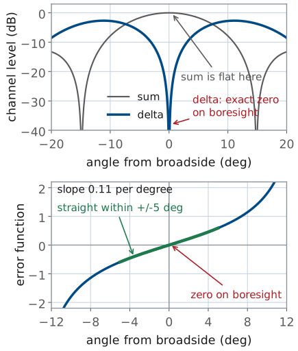
The sum is flat at boresight; the delta climbs out of a zero.
Their ratio turns one look into a signed angle.
Every measurement so far has come from a sweep: the array steps its commanded angle across the field of view and records power at each step. A sweep takes time, and a tracking radar does not have it. Monopulse forms both beams at once from the two subarray channels, adding them for \(\Sigma\) and subtracting them for \(\Delta\). The sum beam is flat at its peak, so its level barely changes as the target drifts a degree off axis. The delta beam is zero on boresight and climbs steeply out of that zero, so its level changes a great deal over the same degree. Dividing one by the other turns that small angle into a large, readable number.
The Error Function
Zero on boresight, with opposite signs on the two sides.
Slope 0.11 per degree, straight within about ±5°.
The two subarrays sit four elements apart, so \(\Delta\) arrives in quadrature with \(\Sigma\), and the useful quantity is the imaginary part of their product. The error function is zero on boresight, positive on one side and negative on the other, and straight within about ±5°, well inside the array’s 13° beamwidth. A target one degree off axis reads about 0.11, and a tracker that drives that reading back to zero holds the beam on the target far more finely than the beamwidth alone would allow, from one look and with no sweep.
The GUI plots a normalized form of the same comparison, taking its sign from the phase difference between the two channels and its magnitude from the two channel levels in dB,
so the trace stays bounded and on screen however strong the target is.
Bench Rules
Open Lab Presets before you press one; Calibrate, then Find HB100.
Set Rx Gain for an FFT peak of \(-10 \pm 3\) dBFS.
Source 1.2 m out, at patch height; facing the patches, E1 is on the right.
The rules come from the Module 3 dry runs. A peak near −10 dBFS keeps the receiver linear with room above the floor; at Rx Gain 10 dB the FFT peak read +2 to +3 dBFS at these distances and the receiver clipped. Every prediction uses the frequency Find HB100 reports for your kit, not the nominal 10.525 GHz; the kits sit anywhere from 10.41 to 10.46 GHz. Level comparisons need the source at 1.2 m or more, because closer in the residual curvature across the aperture puts errors of a few tenths of a decibel on every peak.
Before Every Sweep
Keep ±40° of the bench clear of walls and people.
Recalibrate if the uniform trace is lopsided.
Signal BW resets after Calibrate, Find HB100, or a preset: check it.
In the phaser-00 dry run, a wall beside the kit produced a lobe at −37° to −41° only 9 dB below the peak, and a person seated beside the kit left a −17 dBc shelf on that side. Either one fills a notch. A stale calibration made the uniform trace’s two first sidelobes read unequal, and recalibrating fixed it. Signal BW returned to zero after each of Calibrate, Find HB100, and the Rectangular preset, so check it before every sweep you record.
Equipment and Setup
You need the ADALM-PHASER kit with its Raspberry Pi and Pluto attached, the HB100 source and its battery, a laptop on the same network, and a 1.2 m arc taped on the bench with marks every 15°.
Place the HB100 at boresight, 1.2 m from the array face, at patch-row height and aimed at the center of the patch row. Keep ±40° of the bench clear of walls and people.
Power the PHASER, wait for the Pi to boot, and open
http://phaser.local:8080in a browser.Press Calibrate under Configuration and let it finish. Then press Find HB100 and record the Signal Freq it reports; Part 1 of the packet uses it.
Set Rx Gain so the FFT peak, beam at 0° and source at boresight, reads \(-10 \pm 3\) dBFS. Leave it there for the whole lab.
Check Signal BW, which Calibrate and Find HB100 reset.
Open the Lab Presets section before pressing any preset in it.
No Hardware?
Note
Run the backend in simulation mode with python phaser_headless.py --sim, or
use the hosted simulator, and open the same URL. The simulator places a target
at boresight, so procedures A, B, and D run as written: the weights, the notch,
the difference null, and the error function are all in its physics model. It
also carries a simulated interferer, so procedure C runs there too.
Procedure A: The Static Notch
With the array uniform (Element Gains at 100 %, Phase Control reset), press Start. Read Peak Gain and Angle (set to Peak), then press Freeze to hold the trace as your reference. Record the level of the sidelobe nearest +22.5°; expect about −13 dBc. If the two first sidelobes differ by more than about 2 dB, recalibrate and repeat this step.
Enter your Part 1 gains into Element Gains (Rx1 through Rx8). The set is symmetric, so Enforce Symmetric Taper makes no difference to it; leave the switch off so that a later edit to one slider is not mirrored onto its partner.
Enter your Part 1 phases into Phase Control, each with its sign.
Press Start and read the new trace against the frozen one: the new Peak Gain, the notch’s depth below the frozen peak, and the notch’s angle. Fill in Table A of the packet.
Press Reset in Phase Control and return Element Gains to Uniform.
Procedure B: The Difference Null
Open Digital Beam Forming and set Mode to Manual.
Leave Beam 0 Gain and Phase alone. Set Beam 1 Phase to 180°.
Press Start. Nothing in the analog beamformers changed; only one digital channel’s sign did.
Record the null’s depth and angle, and the angles of the two peaks that replace the main lobe, in Table B. The peaks fall on the sweep’s 2.8125° grid, so one grid step is the reading tolerance.
Set Beam 1 Phase back to 0°.
Procedure C: MVDR Against an Interferer
The interferer in this procedure is simulated: the Phaser software adds a second source, at an angle and level you choose, to the real samples the kit receives, before the digital beamformer sees them. The target stays your HB100 at boresight. Every number in this procedure comes from the two readout tiles under the plot, Interferer vs Target and MVDR Suppression, and from Peak Gain, with the beam held on the target.
Set Mode to Signal vs Time with Steer Angle at 0°. This holds the beam on the target, and the readout tiles fill in only while it is held.
Open the Interferer pane, below Digital Beam Forming, and press Inject Interferer; it changes to Interferer ON · click to stop. Set Angle (deg) to +20 and Power (dBFS) to 0, its maximum, which puts it about 10 dB above a target read at −10 dBFS. Leave Offset from target (kHz) at 100 and Coherent with target off.
In Digital Beam Forming, set Mode to Manual. Watch ten updates of Interferer vs Target and Peak Gain and record the median of each, the middle value once sorted. The readings jump between updates, and the median ignores the odd wild one where an average would not.
Set Mode to MVDR, Snapshots to 1024, and Diagonal Load to 0.1. Leave Steer Angle at 0°: it is MVDR’s look direction. Record the medians of Interferer vs Target, Peak Gain, and MVDR Suppression. The suppression tile needs a Manual and an MVDR reading at the same Steer Angle; if it shows “–”, repeat step 3, then this step.
Open the Adaptive tab, which appears with MVDR in Signal vs Time. Record the angle and depth of the null near +20°, and the conventional pattern’s level at the same angle.
Move the interferer to +30°. Record Peak Gain in Manual, then in MVDR at Diagonal Load 0.001 and at 0.1.
Press the interferer button to turn it off, and set Mode back to Manual and Beam Sweep.
On phaser-00, with the interferer at +20°: Interferer vs Target read about −2 dB in Manual and −18 dB under MVDR, a suppression near 17 dB (single readings from 11 to 20 dB), and the Adaptive tab put the null at 19° to 20°, well below the conventional pattern’s −13 dB. Peak Gain under MVDR reads about 2 dB below Manual, because with the interferer on Peak Gain is the in-band level, and in Manual it includes an interferer only 2 dB below the target. At +30°, loading 0.001 let MVDR cut the target by about 10 dB and 0.1 held the loss near 2 dB; MVDR Suppression read negative at every loading there, MVDR doing worse than Manual.
Procedure D: Watch It Track
Open Lab Presets and load 8 Tracking. It sets the digital layer up to form both beams at once.
Set the taper to Uniform under Element Gains, and check that Beam 1 Phase reads 0° in Digital Beam Forming. The preset resets the phase but not yet the taper, and a leftover taper changes every reading below.
In Plot Options, turn on Show Monopulse Delta Beam and Show Monopulse Error Function.
On the Rectangular tab, press Start. The sum trace peaks on boresight and the delta trace nulls there. Record the delta null’s depth and angle, and the angle where the error trace crosses zero, in Table D.
Open the Tracking tab and press Start. Its y-axis is the steering angle, plotted against sweep count. Move the HB100 slowly across the front of the array along the 1.2 m arc. The tracker reads the error function, drives it back toward zero, and follows the source without sweeping. Note in Table D how far it follows and how it fails when it loses the source.
On phaser-00 the tracker followed smoothly to about ±45°. Near ±48° it lost the source and snapped to the ±90° limits, or to a sidelobe near +60° to +70°, rather than drifting; once the source came back inside about ±45° it locked on again within one sweep.
Lab Packet
The packet is the turn-in document for the whole lab: Part 1 before the period, Part 2 at the bench, Part 3 after. L24 Lab packet (PDF).
Summary
Idea |
What it is |
Number to remember |
|---|---|---|
Weight subtraction |
\(\mathbf{w} = \mathbf{w}_\text{d} - r_\text{n}\mathbf{w}_\text{n}\), as gain % and phase |
main lobe drops about 2 dB for a null at +22.5° |
Notch depth |
set by one-step channel errors, not by rounding, until the room limits it |
about −48 dB; phaser-00 −46 to −50 dB open, −22 to −24 dB cramped |
Difference beam |
Beam 1 Phase \(= 180^\circ\) subtracts the two channels |
boresight null, peaks near ±11°; phaser-00 −41.5 dB open, −22 dB cramped |
MVDR |
\(\mathbf{w} = \mathbf{R}^{-1}\mathbf{s} / (\mathbf{s}^{H}\mathbf{R}^{-1}\mathbf{s})\) from \(K\) snapshots |
one null from two channels; phaser-00 about 17 dB at +20°, \(K = 1024\), loading 0.1 |
Monopulse error |
signed ratio of delta to sum, from one look |
zero on boresight, slope 0.11 per degree |
Looking Ahead
Turn in the packet, all three parts, before Lesson 25.
Module 4 begins radar: the range equation puts a power budget behind this angle measurement.
Lesson 25 derives the radar range equation and asks the question this module never had to: how much power comes back from a target that transmits nothing of its own. Everything Module 3 built, beamwidth, sidelobes, scan loss, and steering, becomes the antenna terms in that equation, and the array you have been sweeping becomes the front end of a radar. The monopulse pair of Part D measures a target’s angle from a single look, which is what a radar needs to track something that moves; the range equation supplies the signal that feeds it. Keep your Table D numbers: the slope of the error function near boresight sets how finely a tracking radar can measure angle, and Module 4 returns to it.