Lesson 20 derived the beamwidth and sidelobe results this lab tests. Today they go to the bench. You sweep the array three times, shrinking the active aperture by half between sweeps, and read the half-power beamwidth, the first-null beamwidth, and the first sidelobe level off each trace. A fourth sweep leaves only the two end elements on, which tests the array factor on a configuration that is not a contiguous block. You compute the predictions before the period, at your own kit’s frequency, so the work at the bench is the third step: reconciling what the plot shows with what the array factor says. Most of the differences have a known cause. One of them, the size of the peak step between apertures, does not yet, and the lab records it as an open measurement.

The PHASER is an 8-element linear array with element spacing \(d = 14\ \text{mm}\). This page works its numbers at 10.3 GHz as one example. There the wavelength is \(\lambda = 29.1\ \text{mm}\), so \(d/\lambda = 0.481\) and the full aperture is \(Nd = 112\ \text{mm}\), just under four wavelengths. Your HB100 runs at its own frequency, somewhere between 10.1 and 10.7 GHz, so your numbers will differ: you will press Find HB100 at the bench, record the Signal Freq it reports, and compute \(\lambda\), \(d/\lambda\), \(kd\), and every prediction at that frequency. The kit in the dry run read 10.408 GHz, where \(\lambda = 28.82\ \text{mm}\).

Two results from Lesson 20 set every number you are about to measure: the half-power beamwidth and the first-null beamwidth above. Both depend on the array only through \(Nd\), the active aperture. Turning off elements at the ends of the row shortens \(Nd\) without changing \(d\), and that is the whole experiment: halve the aperture, watch the beam double. The 0.886 rule carries a small-angle approximation, so check at each aperture whether the beam is narrow enough for it, and solve the array factor’s half-power point directly where it is not.

The table lists the three apertures you will sweep: 8 is E1 to E8, 4 is E3 to E6, and 2 is E4 and E5. The beamwidth columns on Part 1 of the packet are yours to compute at your own frequency. Note that the sidelobe entries are not the same number. The familiar −13 dB figure is the large-\(N\) limit of the uniform array factor. An 8-element array lands at −12.8 dB, close enough to call −13 dB, but a 4-element array reaches only −11.3 dB. The two-element entry is yours to work out from its array factor.

Two entries in the table need care before you go to the bench, and both are in the two-element row. The \(0.886\ \lambda/(Nd)\) rule carries a small-angle step inside it, and the wider the beam, the worse that step gets. Decide whether a two-element beam is narrow enough for it. For two elements the array factor is just \(\cos(\psi/2)\) with \(\psi = kd\sin\theta\), so you can also solve its half-power point directly at your own Signal Freq.

The first-null beamwidth and the first sidelobe come from the same function. The first null of \(\cos(\psi/2)\) needs \(\psi = \pi\), which is \(\sin\theta = \lambda/2d\). Evaluate that at your own Signal Freq and decide whether a real angle satisfies it. Part 1 of the packet asks you to explain what you entered for the two-element FNBW and first sidelobe, and why.

The fourth sweep leaves only E1 and E8 on. It is still a two-element array, so its array factor is the same \(\cos(\psi/2)\) as the E4 and E5 pair, with the spacing \(D = 98\ \text{mm}\) in place of \(d\). That one change tests the derivation on an array that is not a contiguous block, which is what “an arbitrary linear array” in the objective asks for. Work out where \(\psi = 2\pi m\) lands in visible space, and how wide the lobe at 0° is, before you sweep. Compare both with the E4 and E5 row: the two pairs add the same two voltages, so their peaks should agree, and their beams should not. Lesson 23 names what you will see.

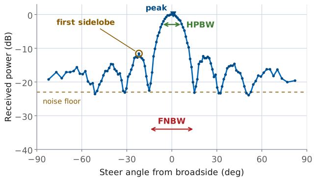
The Rectangular tab does not plot the array factor. It plots received power against commanded steer angle: the software steps the beam past a stationary source and records the power at each step. By reciprocity that traces the array pattern, but three properties of the measurement are baked into every trace you will read.

The sweep is sampled, not continuous. With Use Bits on, as in every lab preset, the software steps the element-to-element phase one ADAR1000 LSB, 2.8125°, per point. One step moves \(\sin\theta\) by \(2.8125^\circ/173.2^\circ = 0.0162\) at 10.3 GHz, which is 0.93° of angle at broadside and 1.32° at 45°, widening as \(1/\cos\theta\). A sweep is 162 points: 123 of them span ±82°, and the other 39 ask for more phase than any real angle needs and plot at ±90°. A feature narrower than one step can fall between samples entirely. The trace has a floor. With all eight elements on, the trace stops following the array factor about 23 dB below the peak of the uniform beam, and anything the array factor puts below that line reads as the floor instead. The floor is not one fixed level for every trace. In the dry run the four-element nulls filled to about −23 dBc of their own, lower peak, while the two-element trace fell about 27 dB from its peak toward the edges of the scan. And the nulls are the first casualties of both effects together: a true null is infinitely deep and infinitely narrow, so the grid usually misses its bottom, and even a sample that lands on it reads the floor.

Per bench:

• ADALM-PHASER (CN0566) with its ADALM-Pluto, on its stand, with its 5 V supply and network connection.

• HB100 Doppler module with a fresh battery, on a tripod.

• A laptop with a browser pointed at http://phaser.local:8080.

Place the HB100 at boresight, about 1 m from the face of the array, at the same height as the patch row and with its face square to the array. Boresight placement matters more than distance in this lab: every prediction is a broadside number, and a source offset by a few degrees shifts the whole trace along the angle axis.

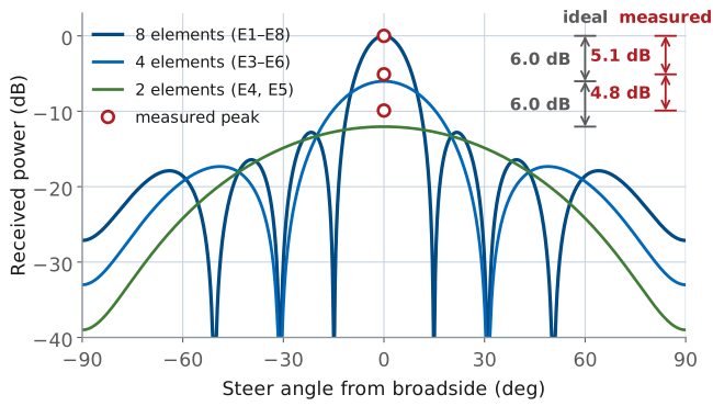
The figure draws the ideal array factor for each aperture at 10.408 GHz, the Signal Freq of the kit in the October 2026 dry run, and marks the three peaks that kit measured. The beam doubles at each halving as Lesson 20 predicts, and the eight- and four-element beamwidths the kit measured land within half a degree of the curves. The peaks do not. The voltage sum predicts steps of 6.0 and 6.0 dB; the kit read 5.1 and 4.8 dB, 9.9 dB in all against 12.0. Expect about \(5 \pm 1\ \text{dB}\) per halving on your own kit.

The cause of that shortfall is not yet known. Two explanations were tested on the dry-run kit and ruled out. Signal leaking through the elements set to 0 accounts for at most 0.5 dB: with all eight gains at 0 the peak fell 33.5 dB below the full array. Receiver compression is ruled out too: lowering every element gain from 100 to 50 lowered the signal, and the shortfall grew, where compression would have made it shrink. The remaining candidates are still being measured, and Part 3 of the packet asks you to propose one with a test that would check it.

None of this touches the shape measurements. HPBW, FNBW, and sidelobe level are all read relative to each trace’s own peak, so an error in the peak level does not move them. The dry-run kit’s eight- and four-element beamwidths landed within half a degree of the array factor at its own 10.408 GHz; its sidelobes and peak steps:

The two-element HPBW is the one shape entry that does not agree. The dry-run kit read it about 6° narrower than the array factor, with a spread of about ±3°, so record it with its spread rather than as a match.

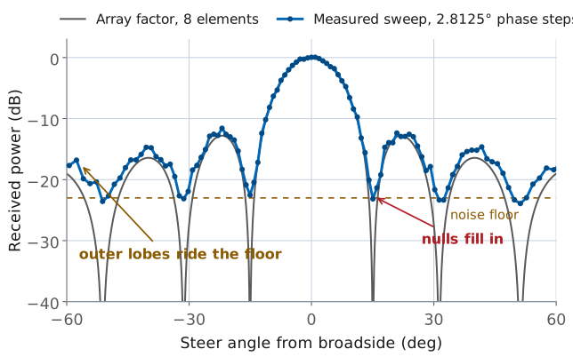
Three differences between your trace and the array factor are expected, and each one has a number attached to it.

The floor sits at about −23 dBc. The trace stops following the array factor about 23 dB below its own peak. Every feature of the array factor below that line — the deep parts of the nulls, and every sidelobe of a tapered array — reads as noise instead of as pattern. This is the usable dynamic range of the measurement, and it is why the lab asks for the first sidelobe rather than the second or third.

Nulls read about −23 dBc instead of \(-\infty\). Two effects fill them, and it is worth keeping them separate. Grid straddle is the smaller one. The 8-element null sits at a phase step of \(360^\circ/8 = 45^\circ\), exactly 16 LSBs, so with the source on boresight a sample lands on it. A source half a step off boresight, 0.47°, leaves the nearest sample at −30 dB, still below the floor. The floor is what fills the null: it adds its own power to every sample near it. Reading each null at its lowest sample puts the measured FNBW up to one step, about 1°, wider than the array factor’s value. The dry-run kit’s eight-element FNBW matched the array factor to within 0.1°.

The first sidelobe reads −11 to −14 dBc. The array factor puts it at −12.8 dB and 21.9°, a phase step of 64.7°. The sample at 23 LSBs, 64.69°, catches it within a hundredth of a decibel, so grid straddle costs nothing here, but the floor adds power to a sidelobe that is only 10 dB above it and noise moves the reading a few tenths either way from sweep to sweep. The two first sidelobes need not match each other either: the dry-run kit read −12.5 dBc on one side and −14.0 dBc on the other. A single number is not meaningful at this dynamic range; a range is.

The half-power readings get less certain as the aperture shrinks. At eight and four elements the dry-run kit’s HPBW landed within half a degree of the array factor. At two elements it read about 6° narrower, with a spread of about ±3°. The two-element pattern is flat near its half-power points: at 10.408 GHz it falls only about 0.2 dB per degree there, against about 1 dB per degree for eight elements. An error of 0.6 dB in the level you read the −3 dB crossings against moves each crossing about 3°, and the HPBW twice that. Report the two-element HPBW with its spread, and expect agreement within several degrees, not within one.

Every trace you took today plots received power against the angle you asked the beamformer for, with the source fixed, so the element pattern contributed the same constant to every point and dropped out of the shape. Lesson 21 puts it back: the patches have their own pattern, and the array radiates the element pattern times the array factor. Keep your three frozen traces. The L21 Lab measures the full pattern by moving the source instead of the beam, and the far edges of today’s eight-element trace are where the two part company.