Printing

To print the slides, switch to present mode and print: one slide a sheet, with room for notes. Print from read mode for the whole lesson.

Equipment and Setup

You need the ADALM-PHASER kit with its Raspberry Pi and Pluto attached, the HB100 source and its battery, a laptop on the same network, and a 1.2 m arc taped on the bench with marks every 15°.

1. Place the HB100 at boresight, 1.2 m from the array face, at patch-row height and aimed at the center of the patch row. Leave it there for all of Part 1: every number there is a comparison between tapers, so the source must not move. Keep ±40° of the bench clear of walls and people.

2. Power the PHASER, wait for the Pi to boot, and open http://phaser.local:8080 in a browser.

3. In the sidebar, press Calibrate under Configuration and let it finish. An uncalibrated array carries element-to-element gain and phase errors that look exactly like a taper you did not ask for. Then press Find HB100 and record the Signal Freq it reports.

4. Set Rx Gain so the FFT peak, beam at 0° and source at boresight, reads \(-10 \pm 3\) dBFS. Leave it there for the whole lab.

5. Open the Lab Presets section, then press 3 Tapering. This loads the Configuration values for the HB100 and selects the Rectangular plot tab.

6. Under Element Gains, confirm Enforce Symmetric Taper is on. With it on, moving one slider moves its mirror-image partner, which is what you want for every taper in this lab.

No Hardware?

Step (a): The Uniform Reference

Press the Uniform taper preset, confirm all eight sliders read 100%, and press Start. Read Peak Gain and Angle (set to Peak), then press Freeze to hold this trace. It stays on the plot as your reference for the rest of the lab, and every peak drop you record is measured against it.

Record the uniform HPBW by reading the angles where the trace falls 3 dB below its own peak. Expect about 13°, within a degree of the 13.1° prediction — the sweep steps in 2.8125° increments, so the 3 dB crossings land between samples. Read the floor, too, and write it at the top of Part 2. If the two first sidelobes, near ±22°, differ by more than about 2 dB, recalibrate and repeat this step.

Step (b): Hann

Press the Hann preset. Before sweeping, do three things:

1. Read the eight slider values and copy them into your table. They should read 12, 43, 77, 100, 100, 77, 43, 12.

2. Compute \(\sum a_n\) and predict the peak drop from \(20\log_{10}(\sum a_n/N)\).

3. Write down the predicted HPBW, 18.9° at 10.443 GHz, or your own from Part 1.

Now press Start. The main lobe should widen from about 13° to about 19°, the peak should sit about 4.7 dB below the frozen uniform trace, and the first sidelobes that were plainly visible at ±22° should be gone into the floor. On an older install expect a milder result, near 17° and −3.7 dB. Record the peak drop, the HPBW, and “below the floor” for the sidelobe level.

Step (c): Blackman and Chebyshev

Repeat step (b) for the Blackman and Chebyshev presets, predicting before each sweep. These two tapers pull the end elements down to 6% and 4%, so most of the array’s outer aperture is barely contributing: the beam widens past 21° and the peak drops past 6 dB, for sidelobes that were already invisible after Hann. This is the point of diminishing returns that Lesson 22 described: a further 2.5° to 3.7° of beamwidth, with no sidelobe improvement this measurement can see.

Step (d): Design Your Own Taper

With Enforce Symmetric Taper still on, design a taper of your own against this specification:

HPBW no wider than 17°, with the first sidelobe below −20 dBc.

Start from Uniform and pull the two end elements down together, leaving the middle elements high. Put the end elements near 25% to 30% and step the elements between them smoothly up to 100%: 30, 55, 90, 100 is a good start. Work by iteration — set the sliders, press Start, read the HPBW and the sidelobe level, and adjust. Two or three passes will get you there.

With a linear slider, 30, 55, 90, 100 predicts 16.5° of beamwidth, a peak drop of −3.3 dB, and a first sidelobe at −25 dBc. On an older install the phaser-00 test run’s 25, 50, 90, 100 read 16.2°, −2.8 dB, and −23 dBc, while end elements at 45% gave −18 dBc and missed the specification. Record your final eight gain values and the measured result in the packet.

Step (e): Restore

Press the Uniform preset before you move on, so Part 2 starts from a known state.

Step (f): Grating Lobes

Leave the source at boresight. With the Uniform preset loaded, check that the frozen uniform trace from step (a) is still on the plot; if it is not, press Start and Freeze again, because it is the reference every peak drop below is read against.

Turn Enforce Symmetric Taper off (the gain lists below are not symmetric) and press Lab preset 4 Grating Lobes. It leaves Rx1, Rx4, and Rx7 at 100% and the other five at 0%, so the three active elements sit \(3d = 42\ \text{mm}\) apart. Press Start. Expect three lobes of the same height: the main lobe at 0° and two copies near ±43°. Read their angles, their heights against the 0° lobe, and the peak drop against the frozen uniform trace.

Now set Rx4 and Rx7 to 0% and Rx5 to 100%, so only Rx1 and Rx5 are on and \(d_\text{eff} = 4d = 56\ \text{mm}\). Sweep again. Expect lobes near ±31°, and the trace climbing to full height at both ends of the plot: the \(m = 2\) solution needs \(\sin\theta\) just past 1, so you see its shoulder rather than its peak.

Step (g): Beam Squint

Move the HB100 to 45° on the 1.2 m arc and press Uniform. Set Signal BW to 10 MHz, press Start, read Angle (set to Peak; it should report the source, about 45°), and press Freeze. Then press Lab preset 5 Beam Squint, check that Signal BW reads 500 MHz (Calibrate, Find HB100, and the Rect preset all reset it to 0), and sweep again. The peak moves even though the source did not.

A beam commanded to \(\theta_c\) with its phases set at \(f_0\) points at \(\sin^{-1}[(f_0/f)\sin\theta_c]\) when the signal is at \(f\). With \(f = 10.443\) GHz and \(f_0 = 9.943\) GHz, the sweep lands on a source at 45° only when it commands 48.0°.

Step (h): Phase Quantization

Put the HB100 back at the arc’s −90° end and press Lab preset 6 Quantization. It holds the beam at 15° with the Blackman taper and opens Signal vs Time on the Tracking tab. With Use Bits checked, set Phase Shift Bits to 7, then walk the HB100 from −90° to +90° along the 1.2 m arc, aimed at the array, in about 20 s. The trace keeps the last 30 s, counted from when the mode starts, so begin walking promptly; a slower walk runs off its end. Read the main-lobe peak and the strongest lobe outside the main lobe. Repeat at 4, 3, and 2 bits, checking the bit count and the box before each walk.

The expectations come from rounding a 15° ramp onto each grid, and the phaser-00 walks of 2026-10-25 matched them: the floor at 7, 4, and 3 bits, and at 2 bits a lobe 10 dB down near −53°, about 2 dB under the −8 dBc prediction, which a hand walk can easily miss by. The 2-bit trace also stays raised, about −11 dBc, over the first stretch of the walk, −90° to −75°. The earlier version of this step swept the beam with the bits reduced and read −15.5, −12.0, and −8.5 dBc at 4, 3, and 2 bits, above both the rule and Lesson 23’s worst-case simulation. Lobes at 3 or 4 bits in the walk would point to the kit rounding more than the steering ramp.

Step (i): Restore

Before you leave: Use Bits on, Phase Shift Bits 7, Signal BW 10 MHz, and the Uniform preset.

Working the Hann Numbers

Work the Hann preset all the way through. The eight amplitudes are \(a_n = 0.12,\ 0.43,\ 0.77,\ 1.00,\ 1.00,\ 0.77,\ 0.43,\ 0.12\), giving

The plotted peak drop follows from the first sum alone:

The directivity loss follows from both sums:

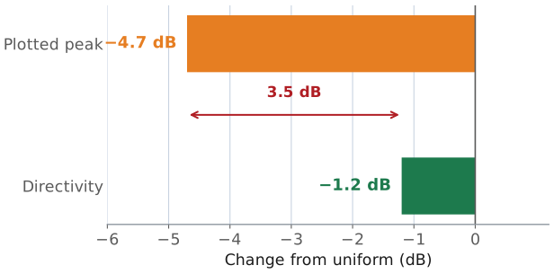
So the trace drops 4.7 dB and the antenna loses 1.2 dB of directivity. The remaining 3.5 dB did not go anywhere, because it was never a loss. The sweep plots received power normalized to full scale, and the tapered array collects less signal voltage from the source — that part is real and it is the 4.7 dB. But the tapered array also responds to less of everything else arriving from off-boresight, and the noise-equivalent aperture shrinks along with the signal sum. Directivity is the ratio of on-axis intensity to the average over all angles, and that ratio only falls by \(\eta_t\). If you re-normalized each trace to its own peak instead of to the uniform peak, the 4.7 dB would vanish from the plot entirely and the beam shape would be unchanged.

The practical statement is short. The peak drop is a plot artifact of a common reference; the taper efficiency is the antenna’s actual loss. A system budget that debits 4.7 dB for the taper overstates the loss by a factor of two in power.

Lab Packet

The packet is the turn-in document for the whole lab: Part 1 before the period, Part 2 at the bench, Part 3 after. L22–L23 Lab packet (PDF).

Summary: Tapering

Summary: The Three Departures