L7 - Simple Resonant Antennas#
Simple Resonant Antennas
Today we extend the math to real hardware.
Lesson 7 · Antennas, Phased Arrays, and Radar Systems · Dr. Neil Rogers
Printing
To print the slides, switch to present mode and print: one slide a sheet, with room for notes. Print from read mode for the whole lesson.
Learning Objectives
- I can describe the radiation behavior of simple resonant antennas (isotropic radiator, half-wave dipole, monopole, loop) and calculate their gain and impedance.
Lesson 6 built the machine: assume a current on a structure, push it through the radiation integral, and out comes the far-field pattern. Today you will extend the math to real hardware. Two antennas form the foundation of the lesson — the isotropic radiator, which cannot be built but which every gain number on every datasheet references, and the half-wave dipole, which you can build with basic tools and which you will be simulating next lesson. By the end of this lesson, you will be able to pick a frequency, cut a wire to length, and predict its pattern, its gain, and what a network analyzer will read at its terminals.
Where We Were
Lesson 4: reflection coefficient
Lesson 5: far field starts at \(r \ge 2D^2/\lambda\).
Lesson 6: radiation integrals
Lesson 5 told us where the far field starts, and only there does the pattern stop changing with range. Lesson 6 gave us the radiation integral: assume a current, transform it into the radiation vector \(\mathbf{N}\), and read the pattern from it. The radiation intensity goes as the square of the transverse part of \(\mathbf{N}\), the field pattern \(\vert F\vert\) is the square root of the intensity normalized to its peak, and directivity compares that peak to the average over the sphere. Lesson 6 also handed us the half-wave dipole pattern from an assumed sinusoidal current. Lesson 4 gave us matching, VSWR, and baluns. Today we need all of these on the same antenna.
Element Factor and Space Factor
We measure \(\vert F(\theta)\vert\).
The element factor is one element’s pattern, here \(\sin\theta\).
The space factor \(S(\theta)\) is the pattern of the current distribution.
Today the integral gives \(S(\theta)\), and the projection supplies \(\sin\theta\).
Lesson 16 calls \(S(\theta)\) the array factor.
Lesson 6 closed on this factorization, and we use it once today, in Step 3 of the pattern derivation. The radiation integral over the sinusoidal current is the space factor of that distribution. Projecting \(N_z\) onto the observer’s transverse direction multiplies by \(\sin\theta\), which is the element factor of every short piece of the wire. Module 3 keeps the same product with a sum in place of the integral. The element factor becomes the pattern of the antenna at each position, and the space factor becomes the array factor, the part of the pattern you steer.
The Isotropic Radiator
It cannot be built: separating charge curves the field lines, so somewhere the field vanishes, and every real antenna has a null.
dBd and EIRP are ratios against the same 0 dBi reference:
An isotropic radiator radiates equally in every direction. Wrap a sphere around it and every square meter of that sphere receives the same power density. Its radiation intensity is simply the radiated power spread over the whole sphere, so its directivity is exactly \(D = 1\), which is 0 dBi — the “i” is literally there to say relative to isotropic.
An isotropic antenna is a physical impossibility. In order to create an antenna, we have to separate charge, which inherently produces curved electric field lines, which means at some physical location the field has to vanish, and a place where the field vanishes is a null.
Every real antenna has at least one null; that is simply a requirement of the physics. The isotropic radiator has no nulls, so it is not an antenna — it is a unit of measurement.
Quantity |
Definition |
Reference |
|---|---|---|
dBi |
gain over an isotropic radiator |
the fiction |
dBd |
gain over a half-wave dipole |
a real antenna |
EIRP |
\(P_t G_t\), transmitter and antenna as one number |
the fiction |
The gain of this theoretical antenna is most useful as a unit of measurement. Recall that dB is a power ratio, so directivity, gain, and effective aperture are all defined as ratios against isotropic. This is why a horn is “16 dBi” rather than “16 dB”. Two related conventions come out of the same reference. Because a half-wave dipole is 2.15 dBi, the two decibel scales differ by a constant.
EIRP is the standard measure of antenna power performance. Feeding 5 W into a half-wave dipole produces the same peak power density as feeding \(5 \times 1.64 = 8.2\ \text{W}\) into an isotropic radiator, so the EIRP is 8.2 W, or 39.1 dBm. One number now describes the transmitter and the antenna together, which is exactly what a link budget needs and exactly what the FCC specifies in their licensing regulations.
Note
Watch the units in the wild. “ERP” usually means effective radiated power referred to a dipole, so ERP and EIRP differ by that same 2.15 dB. Confusing the two changes a link budget by 4.3 dB.
The Short Dipole
Pattern: \(\vert F(\theta)\vert = \sin\theta\), a donut broadside to the wire.
HPBW 90°, \(D = 1.5\), which is 1.76 dBi.
Radiation resistance, about \(2\ \Omega\) at \(L = 0.1\lambda\):
On a \(50\ \Omega\) line, \(2\ \Omega\) gives \(\vert\Gamma\vert = 0.92\) and VSWR 25: 85% of the power reflects.
Lesson 6 handled the infinitesimal dipole — a current element so short that the current is essentially constant along it. Its field pattern is \(\vert F(\theta)\vert = \sin\theta\), a donut with its maximum broadside at \(\theta = 90^\circ\) and nulls off the wire ends. Its beamwidth is 90° and its directivity is \(D = 1.5\), or 1.76 dBi. Its radiation resistance, however, is
about \(2\ \Omega\) for a wire a tenth of a wavelength long. \(2\ \Omega\) against a \(50\ \Omega\) line is a hopeless match, and that, not the pattern, is why nobody feeds a short dipole directly.
The Standing Wave
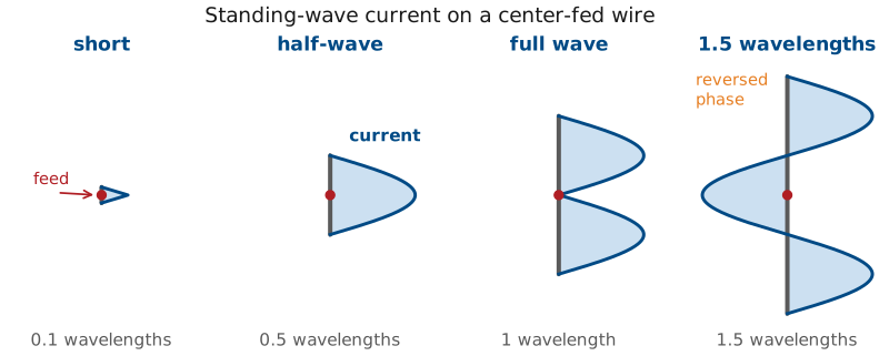
Open-circuited line: zero current at the open end, sinusoidal back toward the source.
Fold the open end apart and the standing wave comes with it:
Tips: \(I = 0\). Feed: a maximum at \(\lambda/2\), a null at \(\lambda\).
Moving away from the infinitesimal wire, the current is no longer a constant as the wire becomes longer. So before we can use Lesson 6’s machinery, we need to understand the effects of a variable current feeding our antenna.
To construct our more realistic dipole, start with a two-wire transmission line, open-circuited at the far end. You already know the mathematical form of its current; on an open-circuited line the current must be zero at the open end. Furthermore, the standing wave varies sinusoidally as you move from the open circuit load back towards the source. At a distance \(s\) back from the open end, the current is:
Now take the open end of that line and fold the two conductors apart until they lie in a straight line, one arm up and one arm down. Congratulations, you have built a center-fed dipole, and it inherits the standing wave that came with it.
Each arm still ends in an open tip. A point at height \(z\) on the upper arm sits a distance \(s = L/2 - z\) back from its tip, so
The lower arm is the mirror image, so replacing \(z\) by \(\vert z \vert\) covers both. Confirm the boundary conditions:
At the tips, \(z = \pm L/2\), the sine argument is zero, so \(I = 0\). Current vanishes at both open ends — charge has nowhere further to go.
At the feed, \(I(0) = I_m \sin(kL/2)\). For \(L = \lambda/2\) that is \(I_m \sin(\pi/2) = I_m\): the current maximum lands exactly at the feed. For \(L = \lambda\) it is \(I_m \sin(\pi) = 0\): a current null at the feed. Remember that contrast — it determines the impedance later in this lesson.
The Current Is the Excitation, Not the Solution
This current is an input, not the solution. It is justified by the transmission-line analogy and confirmed by measurement, but it is not a solution of Maxwell’s equations for a dipole. Everything downstream in this module inherits that assumption.
Measurement and numerical solvers both confirm that the standing wave is very close to the truth for a thin resonant wire. For thick or non-resonant wires it is visibly wrong, and we will be exploring the tradeoffs. The impedance, which depends on the current right at the feed, is where the error shows first.
The Radiation Integral
Step 1: set up and fold. The general integral, then the thin wire along \(z\), then the even current folds onto one arm.
We start with the current, and the radiation integrals of Lesson 6 provide the rest. This is the one antenna in the course where we will run that computation end to end. For a thin wire lying on \(z\), Lesson 6’s radiation vector collapses to one scalar integral,
and the three steps from there are worked in full on the derivation frame below. The radiation intensity goes as \(U \propto \vert N_\theta\vert^2\), so the field pattern is
The result holds within a constant, which is what the proportionality sign is for. The calculus is elementary; the hard part was choosing the current.
Note
The general formula is not a half-wave result. It holds for any \(L\), and the multi-lobe patterns later in this lesson come from the same expression with a different value of \(L\) in it. One integral covers every length, which is the entire purpose of the radiation integral.
Evaluate and Project
Step 2: evaluate, with \(u = kL/2\)
Step 3: project, \(N_\theta = -N_z \sin\theta\)
One integral covers every length.
The product-to-sum identity turns the integrand into two plain sines, both of which integrate directly, and the projection onto the observation direction removes one power of \(\sin\theta\). In the language of the recap frame, the integral is the space factor of the sinusoidal current and the \(\sin\theta\) from the projection is the element factor. The derivation frame below works both steps in full, with \(kL/2\) written out.
Derivation: The Pattern of a Center-Fed Dipole
Step 1: set up the radiation integral. Lesson 6’s radiation vector is
For a thin wire lying on \(z\), the volume integral collapses to a line integral, the current is \(z\)-directed, and \(\hat{\mathbf r}\cdot\mathbf{r}' = z'\cos\theta\):
The current is an even function of \(z'\). Pair each \(z'\) with \(-z'\) and the two exponentials combine into a cosine, which folds the integral onto the upper arm and throws away the imaginary part:
Step 2: evaluate it. This is a relatively straightforward integral. The product-to-sum identity
turns the integrand into two plain sines, both of which integrate directly. Collecting the result:
Step 3: project and normalize. Lesson 6 showed that a \(z\)-directed current radiates only a \(\theta\) component in the far field, obtained by projection: \(N_\theta = -N_z \sin\theta\). That eliminates one power of \(\sin\theta\):
The radiation intensity is \(U \propto \vert N_\theta\vert^2\), and the field pattern is its normalized square root,
That is the pattern of a center-fed dipole of any length, within a constant:
Absolute value and proportionality. Both the proportionality sign and the magnitude bars are there for a reason. The bars matter because for wires longer than \(\lambda\) the bracket changes sign — that sign flip is how sidelobes end up radiating out of phase with the main lobe. The proportionality matters because normalizing means dividing by the peak of that expression, and the peak is not always 1. For \(L \le \lambda\) it sits at broadside, \(\theta = 90^\circ\), where the expression evaluates to \(1 - \cos\dfrac{kL}{2}\); for longer wires the peak moves off broadside entirely, which is the story later in this lesson.
The Half-Wave Dipole Pattern
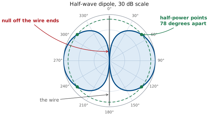
A donut again, slightly narrower than the short dipole’s.
HPBW 78°.
\(D = 1.64\), which is 2.15 dBi.
Set \(L = \lambda/2\), so that \(kL/2 = \pi/2\) and the second cosine vanishes. The broadside peak is then \(1 - 0 = 1\), so this one is already normalized and can be written with an equals sign. This is the half-wave dipole pattern. The \(\sin\theta\) in the denominator looks like trouble at \(\theta = 0\), but the numerator vanishes there too and the ratio goes quietly to zero. The nulls are still straight off the ends of the wire.
Solving \(\vert F(\theta)\vert^2 = 1/2\) numerically gives half-power points at \(\theta = 51.0^\circ\) and 129.0°, so
Integrating \(\vert F\vert^2\) over the sphere gives the directivity,
Copper is a good conductor, so radiation efficiency for a wire dipole is above about 98% and \(G = \eta_{\text{rad}} D\) is within a tenth of a dB of \(D\). For this antenna we can quote gain and directivity interchangeably — but it is still helpful to be in the habit of specifying which one you mean, because for the lossy antennas in Module 4 they diverge significantly.
From Short to Half-Wave
Beamwidth 90° to 78°; directivity 1.76 to 2.15 dBi, up 0.39 dB.
Pattern: how many wavelengths of current fit the wire.
Impedance: where the current maximum sits relative to the feed.
Half a wavelength puts the current maximum at the feed.
Now look at what lengthening the wire from a small fraction of a wavelength to \(\lambda/2\) actually gained us: the beamwidth went from 90° to 78° and the directivity went from 1.76 to 2.15 dBi. Lengthening the wire brought 0.39 dB of directivity.
A dipole’s pattern is set by how many wavelengths of current fit on the wire. Its impedance is set by where the current maximum sits relative to the feed. Half a wavelength is the optimal length because it puts the current maximum right at the feed point, and the pattern is within 0.39 dB of the short dipole’s.
Why Half a Wavelength?
\(73\ \Omega\) is power leaving.
\(+j42.5\ \Omega\) is Lesson 5’s near field, doing no useful work.
Resonance means \(X_{\text{in}} = 0\); we are \(42.5\ \Omega\) away.
The reason to use a half-wave dipole is its input impedance rather than its 2.15 dBi. At \(\lambda/2\) the current maximum sits at the feed, so the feed sees a useful resistance. A short dipole’s \(2\ \Omega\) is hopeless; \(73\ \Omega\) is close enough to a \(75\ \Omega\) line to nearly match it without a network. The resistive part is real radiation. The \(+42.5\ \Omega\) is inductive: stored energy in the reactive near field of Lesson 5, the term that never made it into the far field. Nothing is wrong with the antenna at exactly \(\lambda/2\); it simply is not resonant there, and trimming fixes that.
The next frames show where both numbers come from: the resistance from the pattern we just derived, and the reactance from one standard near-field result that we name but do not re-derive.
The Radiation Resistance
The pattern is only half of the analysis. What the transmitter actually sees is the input impedance, and for a thin half-wave dipole we can calculate both parts of it — the resistance comes from the pattern we just derived and the reactance from one standard result we will name but not re-derive.
Radiation resistance is defined by asking what resistor, carrying the same current, would dissipate the power the antenna radiates. If we can compute \(P_\text{rad}\), we can find \(R_r\). Start from the half-wave pattern, and this time keep the constants. Lesson 6 gave the radiation intensity in terms of the radiation vector,
and for the dipole \(N_\phi = 0\) while Step 3 gave \(N_\theta = -N_z\sin\theta\). With the Step 2 result for \(N_z\) at \(L = \lambda/2\),
Square it and multiply by the Lesson 6 constant. The \(k^2\) cancels, which is why the radiation resistance of a half-wave dipole depends on the shape \(\lambda/2\) and not on the frequency:
The \(\vert I_m\vert^2\) out front is what makes the last step work: dividing \(P_\text{rad}\) by \(\tfrac{1}{2}\vert I_m\vert^2\) leaves a resistance with no current in it.
The radiated power is that intensity integrated over the whole sphere. Nothing depends on \(\phi\), so the azimuth integral simply contributes \(2\pi\):
The Result: 73 Ohms
No elementary antiderivative. The integral is a tabulated number, \(\tfrac{1}{2}C_{in}(2\pi) = 1.2188\), and the current level cancels.
Here the derivation stops being algebra. That integral has no elementary antiderivative. You cannot write the answer in terms of sines, logs, and powers — this is the point where a number enters instead of a formula.
That is not a failure, and it is not unusual. It is the same situation as \(\text{erf}\) in probability: the integral is important enough that somebody tabulated it, gave it a name, and moved on. Antenna work leans on three such special functions, and we will use all of them again:
\(Si\) is the sine integral, \(Ci\) the cosine integral, and \(C_{in}\) the modified cosine integral; the last two are one function apart, \(C_{in}(x) = \gamma + \ln x - Ci(x)\) with \(\gamma = 0.5772\), Euler’s constant. Look them up, or let a calculator evaluate them; do not try to integrate them. The solution function we need for this integral is:
Equate the two expressions for \(P_\text{rad}\); the \(\vert I_m \vert^2\) cancels and the antenna’s current level drops out, as it must. Since \(\eta_0/4\pi = 29.98\ \Omega\), which is \(30\ \Omega\) to better than one tenth of a percent, the result is easy to remember as 30 times 2.4376.
The power calculation used \(I_m\), which is the largest current anywhere on the wire. A resistance referred to that point equals the resistance measured at the feed terminals only when the current maximum is physically located at the feed. For a half-wave dipole it is, so the two numbers agree. For a full-wave dipole they do not: a full-wave dipole has a current minimum at the feed, and its feed resistance is enormous — hundreds to thousands of ohms — even though the current-maximum resistance is a moderate \(199\ \Omega\).
Reactance via the Induced-EMF Method
A far-field power integral counts only power that leaves.
Reactance is near-field energy, so it takes the induced-EMF method.
At \(\lambda/2\), \(\sin kL = 0\) and every wire-radius term drops out.
A far-field power integral can only ever produce the real part — it accounts for power that leaves. The reactance describes cyclical energy in the near field which never crosses the far-field sphere at all, so no amount of pattern integration will produce it.
Finding the reactance requires a different technique. We will use the induced-EMF method, in which we integrate the field the antenna reflects back against its own current, along the wire. That is a near-field calculation, and the derivation frame below sets it up and states its general result. That result contains \(Si\), \(Ci\), and the wire radius \(a\) — meaning that the reactance of a dipole normally depends on how thick the wire is.
At exactly \(L = \lambda/2\) that dependence disappears. Every term containing the wire radius is multiplied by \(\sin(kL)\), and at \(kL = \pi\),
The wire radius factors out, and what survives is a single special function.
The reactance of a dipole is radius-independent only at exactly \(\lambda/2\). That is why \(42.5\ \Omega\) can be quoted as a clean number at all, while at every other length the reactance depends on how thick the wire is — which is exactly why the three curves in the next figure separate everywhere, but cross at \(\lambda/2\).
Put the two halves side by side and the whole impedance is one line, built from two tabulated numbers:
So read the two parts separately. The \(73\ \Omega\) is power leaving and never coming back — the whole point of the antenna. The \(+j42.5\ \Omega\) is the reactive near field of Lesson 5, which does no useful work, and wrecking your match.
Every step above assumed the sinusoidal current from the standing-wave frame. How much that matters depends on what you are computing. The pattern shape barely cares: the radiation integral smooths over small errors in the current, so the 78° beamwidth and 2.15 dBi hold up well. The impedance cares a great deal, because it depends on the current right at the feed and on the near fields close to the wire. This is the main reason a simulator will not return exactly \(73 + j42.5\ \Omega\). Measuring how large that disagreement is, and deciding whether it matters, is the work of Lesson 8.
Derivation: Input Impedance by the Induced-EMF Method
What the method does. The far-field route cannot see the reactance, so this one stays close to the wire. Assume the same sinusoidal current on the surface of a wire of radius \(a\), compute the electric field that current produces along the wire’s own surface, \(E_z(\rho = a, z')\), from the exact vector potential with the full \(1/R\) kernel rather than the far-field approximation, and integrate that field against the current. The result is the impedance referred to the current maximum,
The physical reading is that \(-\tfrac{1}{2}\int E_z I\ dz'\) is the complex power the current delivers to its own field: the real part leaves as radiation, the imaginary part is stored and returned each cycle. Dividing by \(\tfrac{1}{2}\vert I_m\vert^2\) turns that power into an impedance. The integration is long and is in Balanis, Chapter 8; the general result is what matters here.
The general result. With \(\gamma = 0.5772\), Euler’s constant,
Both are referred to the current maximum. The feed sees \(Z_\text{in} = Z_m / \sin^2(kL/2)\), which is the same thing at \(\lambda/2\) and larger for a shorter wire, where the feed sits below the current maximum.
The special functions. \(Si\) is the sine integral, \(Ci\) the cosine integral, and \(C_{in}\) the modified cosine integral, and they are one family:
At \(L = \lambda/2\). Then \(kL = \pi\), \(\sin kL = 0\), and \(\cos kL = -1\). Every bracket multiplied by \(\sin kL\) vanishes, and the wire radius, which appears only inside one of them, drops out. What survives is
The resistance is the same \(73.1\ \Omega\) the far-field power integral gave, from a near-field calculation that shares nothing with it but the assumed current. That agreement is a check on both routes.
Off \(\lambda/2\), the radius matters. Solving \(X_\text{in} = 0\) from the general result gives the resonant length and the feed resistance there:
\(a/\lambda\) |
\(L/2a\) at resonance |
Resonant length |
\(R_\text{in}\) |
|---|---|---|---|
0.0001 |
2400 |
\(0.485\lambda\) |
\(67\ \Omega\) |
0.001 |
240 |
\(0.479\lambda\) |
\(65\ \Omega\) |
0.002 |
120 |
\(0.476\lambda\) |
\(63\ \Omega\) |
0.005 |
47 |
\(0.470\lambda\) |
\(61\ \Omega\) |
0.01 |
23 |
\(0.463\lambda\) |
\(59\ \Omega\) |
A thicker wire resonates shorter, which is the “Why Shorter?” frame with numbers on it. The \(0.002\lambda\) row is the Smith chart widget’s wire, and its \(63\ \Omega\) is the number the chart reads at the resonant crossing. The resistances run below the \(70\ \Omega\) a bench measures because the sinusoidal current is an approximation once the wire is off \(\lambda/2\), and Lesson 8 measures that gap.
Resonance
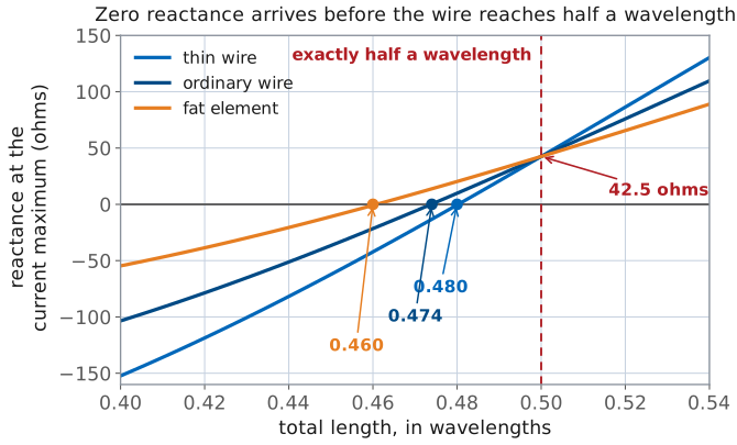
Resonance means \(X_{\text{in}} = 0\).
The fix is to make the wire slightly shorter.
The zero crossing moves lower as the element gets thicker.
All three curves meet at \(\lambda/2\), where \(\sin(kL) = 0\).
At exactly \(\lambda/2\) we are \(42.5\ \Omega\) away from resonance. The figure is computed, not sketched: the induced-EMF impedance evaluated at hundreds of lengths for three wire radii. The reactance passes through zero below \(\lambda/2\) for every radius, and the crossing moves left as the element gets thicker. The next frame says why.
Why Shorter?
End effect: capacitance at the tips lets charge pile up past the metal.
Wire thickness: a thicker element has more end capacitance.
Both slow the wave on the wire.
Resonance lands near \(0.475\lambda\): \(63\ \Omega\) modeled, \(70\ \Omega\) measured.
The reason is that the wire is electrically longer than it is physically.
End effect. Capacitance between the tips of the dipole — and to the insulators, mast, and everything else nearby — lets charge accumulate past where the metal stops. The standing wave behaves as though the wire continued a little further than it does.
Wire thickness. A thicker element has more end capacitance and a lower characteristic impedance, so it shortens further. This is why a thin wire resonates near \(0.480\lambda\) while a thick tubular element can drop to \(0.46\lambda\).
Both effects slow the wave traveling on the wire relative to free space, and a slower wave needs less physical length to fit the same electrical half wavelength. For ordinary wire the answer lands in the range \(0.47\lambda\) to \(0.48\lambda\), and the resistance drops with the length, to roughly \(70\ \Omega\). The induced-EMF derivation frame above tabulates both against wire radius from the general result.
The 5% Rule
Cut a resonant dipole to about 95% of a half wavelength:
Cut it long and trim. You can always remove wire.
The 5% is an average. It depends on wire gauge, insulation, and what is nearby, which is exactly why you trim rather than compute to four digits.
The Match
Line |
Load |
\(\vert \Gamma \vert\) |
VSWR |
|---|---|---|---|
\(50\ \Omega\) |
\(73 + j42.5\), untrimmed |
0.37 |
2.18 |
\(50\ \Omega\) |
\(70 + j0\), resonant |
0.17 |
1.40 |
\(75\ \Omega\) |
\(73 + j42.5\), untrimmed |
0.28 |
1.76 |
\(75\ \Omega\) |
\(70 + j0\), resonant |
0.03 |
1.07 |
Trimming to resonance beats changing the cable. Kill the reactance first; worry about the resistance second.
With a resonant dipole in hand, the match is a one-line calculation. Using Lesson 4’s
the table compares the untrimmed and resonant dipole on each line. On a \(50\ \Omega\) line, removing the \(+j42.5\ \Omega\) of reactance takes the VSWR from 2.18 to 1.40. Leaving the reactance in place and switching to a \(75\ \Omega\) cable only reaches 1.76. Trimming to resonance is worth more than changing the cable.
Resonance on the Smith Chart
Those four rows are the same information a Smith chart shows at a glance, and you will be reading charts for the rest of the course — every VNA in the lab draws one. The chart is the complex reflection coefficient plane. The center is a perfect match, the rim is total reflection, the upper half is inductive and the lower half capacitive.
Four kinds of object are drawn on the chart, and each is worth naming before you touch the slider.
The faint gray grid is the chart itself, printed once and never moving. The circles that all pass through the right-hand point are lines of constant resistance; the arcs curving away from that point are lines of constant reactance. Together they let you read an impedance off any position.
The amber dashed circles are lines of constant VSWR, centered on the match point at 2:1 and 3:1. Anything inside the 2:1 circle is a usable match.
The blue curve is the antenna. It is the impedance locus: the path the dipole’s feed impedance traces as its length \(L/\lambda\) sweeps from one end of the slider range to the other. Each point on it is one antenna, of one particular length. The curve is not part of the chart — it is the data.
The markers call out two lengths on that locus: the red one is exactly \(\lambda/2\), and the green one is the resonant length.
The single most important feature is where the blue locus crosses the horizontal axis. On the horizontal axis the reactance is zero, so that crossing is resonance — it is the same event as the zero crossing in the reactance figure earlier in this lesson, drawn a different way. The resistance you read at that crossing is the radiation resistance of the resonant dipole.
Now use the slider. Find the \(\lambda/2\) marker and confirm it reads \(73 + j42.5\ \Omega\), sitting in the upper (inductive) half and outside the 2:1 circle. Then shorten the antenna and watch the locus walk down onto the axis and inside the 2:1 circle as the VSWR readout falls.
Finally, switch the normalization from \(50\ \Omega\) to \(75\ \Omega\). The antenna does not change and the impedance readout does not change, but the grid re-scales underneath it and the same antenna lands closer to the center. A match is a property of an antenna and a line together, not of the antenna alone. Throughout, the wire is assumed thin — radius \(0.002\ \lambda\) — and only the colors are keyed under the chart; the list above is the full reading of it.
Why the Chart Says 63 Ohms
The chart reads about \(63\ \Omega\) at the resonant crossing.
Real resonant dipoles measure about \(70\ \Omega\).
The first is the sinusoidal-current model on a slightly short wire; the second is what solvers and benches return.
Design with \(70\ \Omega\).
At the resonant crossing the chart reads about \(63\ \Omega\), but this lesson has been telling you to design around \(70\ \Omega\). Both numbers are correct, and the difference is not a mistake in either one.
\(63\ \Omega\) is what this model predicts. Everything in the widget comes from the assumed sinusoidal current above, applied to a thin wire of radius \(0.002\ \lambda\). At exactly \(\lambda/2\) that model is excellent, which is why the chart reproduces \(73 + j42.5\ \Omega\) there to the digit. Shorten the wire toward resonance and the model drifts: the real current on a slightly short, finite thickness wire is not quite sinusoidal, and the model responds by predicting a resistance several ohms low.
\(70\ \Omega\) is what real resonant dipoles measure. It is the number that comes back from method-of-moments solvers and from antennas on a bench, and it is the number to carry into a design.
Use the chart to understand the shape of the behavior — that resonance is a crossing of the real axis, that trimming moves you there, that the locus leaves the useful region quickly on either side. Use \(70\ \Omega\) when you need a number. Lesson 8 is where you measure the gap between the two for yourself.
Balanced Dipole, Unbalanced Coax
A dipole is balanced; coax is unbalanced.
Wired together directly, the shield radiates and the pattern and VSWR depend on where you stand.
Lesson 4’s fix is a balun. Every dipole in this course gets one.
One practical matter remains before you connect anything. Wire a dipole and a coax together directly and current flows on the outside of the shield, the feedline joins the radiating structure, and your pattern and VSWR both start depending on where you are standing. Lesson 4 gave you the fix: put a balun at the feed point.
The Folded Dipole
Two parallel half-wave conductors, joined at both ends, fed in the middle of one.
Same pattern as the half-wave dipole, but about \(4 \times 73 \approx 290\ \Omega\) at the feed.
Usually fed from \(75\ \Omega\) through Lesson 4’s 4:1 half-wave balun.
Bend a second half-wave wire alongside the first, close compared with a wavelength, join the two at both ends, and feed only one of them. You get a dipole with the same pattern and four times the input resistance, and it is common enough (FM and TV antennas, 300 Ω twin-lead, the driven element of many Yagis in Lesson 14, plenty of vertical base-station antennas) that you should know where the four comes from.
Split the feed current into two modes. In the antenna mode the two conductors carry equal, in-phase currents (for equal diameters), so a feed current \(I\) puts \(2I\) on the structure, and the far field sees one half-wave dipole carrying \(2I\). The feed supplies all of that power:
In the transmission-line mode the currents are equal and opposite, so they do not radiate; each half of the fold is a two-wire line a quarter wave long, shorted at its far end, and at resonance that stub is an open circuit that draws nothing. Off resonance its reactance swings the opposite way to the dipole’s and partly cancels it, which is why a folded dipole is somewhat broader-band than a plain one.
The same argument gives \(N^2\) for \(N\) conductors, 9 times for three, and unequal diameters change the ratio, which makes the step-up a design knob for matching. The middle of the unfed conductor sits at zero RF voltage, so it can be bolted straight to a grounded boom or mast: a folded dipole is DC-grounded, which drains static and helps with lightning. Sealed in a radome, it looks exactly like a monopole or a sleeve dipole, and Lesson 12 takes up why that matters when you mount one.
Longer Dipoles Grow Lobes
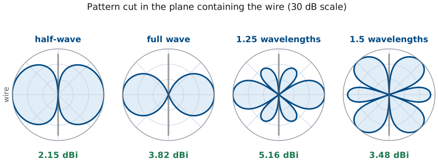
Each phase reversal past \(\lambda/2\) adds a pair of lobes.
Length |
HPBW |
\(D\), dBi |
\(R\) at current max |
|---|---|---|---|
short |
90° |
1.76 |
\(\approx 2\ \Omega\) |
\(0.5\lambda\) |
78° |
2.15 |
\(73\ \Omega\) |
\(1.0\lambda\) |
48° |
3.82 |
\(199\ \Omega\) |
\(1.25\lambda\) |
33° |
5.16 |
\(106\ \Omega\) |
\(1.5\lambda\) |
— |
3.48 |
\(105\ \Omega\) |
Keep stretching the wire past \(\lambda/2\) and the standing wave develops phase reversals: sections of the wire carry current in the opposite direction. Reversed current radiates out of phase with the rest, the contributions interfere, and the single donut breaks into lobes. The radiation integral is linear, so this is exact in the language of the recap frame: a \(1.5\lambda\) wire is three half-wave sections carrying \(+, -, +\), the half-wave pattern is the element factor, and the three sections at \(\lambda/2\) spacing with alternating signs are a space factor, which Lesson 16 would call a three-element array with 180° progressive phase. The element factor’s null on the axis is why the lobes lean toward the wire without reaching it. Below \(\lambda/2\) nothing changes; above \(1.25\lambda\) the main lobes move off broadside, so a single broadside beamwidth is meaningless at \(1.5\lambda\).
The resistance column is referred to the current maximum, and it sweeps through \(50\ \Omega\) twice before the wire is a wavelength long, which is why non-resonant lengths are hard to match.
The Dipole Explorer
Park it at 0.50, back off to 0.474, then switch the wire to fat. The interactive animation is a good way to intuit the effects of length and current distribution on the pattern. Drag the length slider from one end to the other and watch three things at once: the standing-wave current on the wire, the pattern it produces, and the numbers in the pills underneath. Notice that below half a wavelength almost nothing changes — the pattern is essentially the short-dipole donut all the way down to the infinitesimal case. This means an electrically small antenna is an impedance problem and not a pattern problem. Then notice that directivity creeps upward until about 1.2 to 1.25 wavelengths, where it peaks near 5.2 dBi; past that point the main lobe splits and the broadside gain collapses. Park the slider at 0.50 and confirm the canonical trio: 78.1°, 2.15 dBi, \(73.1\ \Omega\). Back off to 0.474 and the reactance crosses zero; switch the wire to fat and resonance moves to \(0.461\lambda\).
Note
The resistance and reactance in the interactive widget are referred to the current maximum, not to the terminals. At \(L = \lambda/2\) the current maximum sits at the feed and the two are the same number, which is the case you care about. For other lengths the terminal values are larger by \(1/\sin^2(kL/2)\) — a short dipole’s tiny current-maximum reactance becomes an enormous terminal reactance, which is precisely why short antennas are so hard to feed.
Cut One for 146 MHz
Quantity |
Work |
Result |
|---|---|---|
Wavelength |
\(c/f\) |
2.055 m |
Half wave |
\(\lambda/2\) |
1.027 m |
Trimmed |
\(0.475\lambda\) |
0.976 m |
Each arm |
\(L/2\) |
48.8 cm |
Check |
\(143/f_\text{MHz}\) |
0.980 m |
The whole design is two 49 cm arms.
Design a resonant half-wave dipole for 146 MHz. The two routes agree to within a centimeter, which is well inside the accuracy of the rule, and 49 cm is a length you can eyeball. The worked example below carries the full calculation.
What the Analyzer Should Read
Quantity |
Prediction |
From |
|---|---|---|
\(Z_{\text{in}}\) |
\(\approx 70 + j0\ \Omega\) |
trimmed |
VSWR on \(50\ \Omega\) |
1.40 |
\(\vert\Gamma\vert = 0.17\) |
VSWR on \(75\ \Omega\) |
1.07 |
\(\vert\Gamma\vert = 0.03\) |
Gain |
2.15 dBi |
\(D = 1.64\) |
\(\theta_\text{HP}\) |
78° |
half-wave pattern |
Far-field distance |
0.93 m |
\(2D^2/\lambda\), Lesson 5 |
Fit the balun, then trust the table.
Every number here is unremarkable, which is what you want. A dipole calculation that returns 12 dBi or \(8\ \Omega\) is outside the physically reasonable range and indicates an arithmetic error. If the analyzer disagrees by more than about 10%, suspect the balun before the theory.
Worked Example: A 2 Meter Dipole for 146 MHz
Worked example — a 2 meter dipole for 146 MHz
Design a resonant half-wave dipole for 146 MHz and predict what the analyzer will show.
Wavelength.
Physical length. A half wavelength is 1.027 m; apply the 5% rule:
Cross-check with the field-manual form: \(143/146 = 0.980\ \text{m}\). The two agree to within a centimeter, which is well inside the accuracy of the rule.
Cut list. Two arms of \(L/2 = 48.8\ \text{cm}\), fed at the center, with a balun.
Predicted performance.
Quantity |
Value |
Where it came from |
|---|---|---|
\(Z_{\text{in}}\) |
\(\approx 70 + j0\ \Omega\) |
resonant, trimmed |
VSWR on \(50\ \Omega\) |
1.40 |
\(\vert\Gamma\vert = 20/120 = 0.167\) |
VSWR on \(75\ \Omega\) |
1.07 |
\(\vert\Gamma\vert = 5/145 = 0.034\) |
Gain |
2.15 dBi |
\(D = 1.64\), copper loss negligible |
\(\theta_\text{HP}\) |
78° |
half-wave pattern |
Far-field distance |
\(2D^2/\lambda = 0.93\ \text{m}\) |
Lesson 5, with \(D = 0.976\ \text{m}\) |
Sanity check. Every number above is unremarkable, which is what you want. A dipole calculation that returns 12 dBi or \(8\ \Omega\) is outside the physically reasonable range and indicates an arithmetic error.
Note
Two of those numbers need a footnote. The sinusoidal-current model used here predicts a resonant resistance in the low sixties; a full numerical solver and a real measurement both land closer to \(70\ \Omega\). And the exact resonant length depends on wire gauge, insulation, and what is nearby. Carry \(70\ \Omega\) and \(0.475\lambda\) as the design numbers, and expect a few percent of disagreement — quantifying that disagreement is what the next lesson is for.
Build It: A 915 MHz Dipole
\(\lambda = 32.8\ \text{cm}\), so \(L = 0.475\lambda = 15.6\ \text{cm}\): 7.8 cm per arm.
Cut long. Solder one arm to the center pin and the other to the body.
Straighten both arms.
Write your predictions down before Lesson 10.
Build it — a 915 MHz wire dipole on an SMA connector
Ten minutes with a wire cutter and a soldering iron gets you a real antenna. You will not measure it today. You will measure it in Lesson 10, on a vector network analyzer, against the predictions you write down now — so the value of this exercise depends entirely on committing to numbers before you cut.
Parts. An SMA female panel-mount or edge-launch connector, about 20 cm of 20 AWG solid copper wire — stiff enough to hold its shape — a wire cutter, a ruler, and a soldering iron.
Design, then build.
At 915 MHz, \(\lambda = c/f = 32.8\ \text{cm}\). The 5% rule gives a total length \(L = 0.475\lambda = 15.6\ \text{cm}\), which is 7.8 cm per arm. The same three lines work for any other band with a new \(f\).
Cut two arms at 7.8 cm. Cut them long if you are unsure. You can always trim; you cannot un-trim.
Solder one arm to the connector’s center pin and the other to the connector body or ground tab, so the two arms run in opposite directions along one straight line.
Straighten both arms and check that the pair is collinear and square to the connector. A bent dipole is a different antenna.
Fill in the prediction column on the next frame and keep the sheet with the antenna.
Fill In Your Predictions Now
What to record |
Your prediction (now) |
Measured in Lesson 10 |
|---|---|---|
Arm length actually cut |
______ cm |
— |
Total length \(L\) |
______ cm |
— |
Resonant frequency \(f_\text{res}\) |
______ MHz |
______ MHz |
Feed impedance \(Z_{\text{in}}\) at resonance |
______ \(\Omega\) |
______ \(\Omega\) |
VSWR on a \(50\ \Omega\) line |
______ |
______ |
This build has no balun, and that matters
Soldering wire straight onto an SMA connector is the crudest possible feed: the dipole is balanced, the coax behind it is not, and current will flow on the outside of the shield exactly as Lesson 4 warned. The feedline becomes part of the antenna. Expect your measured resonant frequency and impedance to drift from the predictions above, and expect the readings to twitch when you move your hand near the cable. That is not a botched build. It is the balun problem showing up in your own hardware.
Key Points
A resonant dipole is about \(0.475\lambda\) long, near \(70\ \Omega\), 2.15 dBi, and 78° wide.
The resistance comes from a far-field power integral; the reactance cannot.
Every number rests on the assumed sinusoidal current. Lesson 8 tests it.
A dipole’s pattern is set by how many wavelengths of current fit on the wire.
Its impedance is set by where the current maximum sits relative to the feed.
Half a wavelength is the optimal length because it puts the current maximum at the feed. It costs only 0.39 dB of directivity to implement.
The resistance comes from a far-field power integral; the reactance does not and cannot.
A resonant dipole is about \(0.475\lambda\), near \(70\ \Omega\), 2.15 dBi, 78° wide.
Every number here rests on the assumed sinusoidal current.
Summary
Symbol / idea |
What it is |
Number to remember |
|---|---|---|
Isotropic radiator |
Equal radiation in all directions; impossible, but the reference for everything |
\(D = 1\), 0 dBi |
EIRP |
Transmitter and antenna as one number, \(P_t G_t\) |
\(\text{dBi} = \text{dBd} + 2.15\) |
Assumed current |
Standing wave from the unfolded open-circuited line |
\(I_m \sin[k(L/2 - \vert z\vert)]\) |
Short dipole |
Constant current, limiting case |
\(\vert F\vert = \sin\theta\), 1.76 dBi |
Dipole pattern, any length |
One radiation integral covers every length; normalize by the peak |
\(\vert F\vert \propto \left\vert\left[\cos\left(\frac{kL}{2}\cos\theta\right) - \cos\frac{kL}{2}\right]/\sin\theta\right\vert\) |
Half-wave dipole pattern |
The general result at \(kL/2 = \pi/2\) |
\(\theta_\text{HP} = 78^\circ\) |
Half-wave directivity |
From integrating the pattern over the sphere |
\(D = 1.64 = 2.15\ \text{dBi}\) |
Special functions |
Tabulated, like \(\text{erf}\) — do not integrate them |
\(C_{in}(2\pi) = 2.4376\), \(Si(2\pi) = 1.4182\) |
Half-wave impedance |
Resistance from the far field, reactance from induced EMF |
\(\frac{\eta_0}{4\pi}\left[C_{in}(2\pi) + jSi(2\pi)\right] = 73 + j42.5\ \Omega\) |
Resonance |
\(X_{\text{in}} = 0\), reached by trimming |
\(0.47\lambda\) to \(0.48\lambda\), \(\approx 70\ \Omega\) |
The 5% rule |
Resonant length from frequency |
\(143/f_\text{MHz}\) meters |
Longer dipoles |
Phase reversals build lobes |
Peak \(\approx 5.2\ \text{dBi}\) near \(1.25\lambda\) |
Practice
Where This Is Going
Lesson 8: the pattern computed numerically, with no current prescribed. Bring the 146 MHz numbers and grade it with them.
Lesson 12: a monopole and a loop from the same wire.
Module 3: the dipole becomes an element.
Lesson 8 puts this exact antenna into nec_lab, the course simulator, which acts as a front end to NEC-2, the Numerical Electromagnetics Code — a method-of-moments engine written in the 1970s and still the standard tool for wire antennas. What it does is compute the radiation pattern numerically, which is the one thing this lesson could not do. It divides the wire into short segments, treats each as a small radiator whose pattern we already know, and adds those patterns up; the weights in that sum come from enforcing the boundary condition that the total tangential electric field must vanish on a perfect conductor, which also hands back the current on each segment along the way. So the simulator is not doing different physics from this lesson. It is running the same superposition without anyone having to prescribe the current first, and that is exactly why comparing the two is informative.
In Lesson 8 you will model a wire, set its length, sweep the frequency, and read back impedance, VSWR, gain, and pattern — then compare each one against the numbers you produced by hand today. The numbers you just predicted are the ones you will check against simulation. A simulator that agrees with a hand calculation on a dipole can be trusted a little further on a structure you cannot solve by hand; a disagreement usually points to a setup error in the model, and the only way to notice it is to bring predictions with you. The 915 MHz dipole you soldered onto an SMA connector closes the same loop with hardware instead of software: in Lesson 10 you will put it on a vector network analyzer and see how far a real balun-less wire lands from the length, resonance, and impedance you wrote down today.
After that, Lesson 12 takes the same wire apart. Cut a dipole in half and stand it on a ground plane and you have a monopole — half the impedance, double the directivity, and only the upper half-space to radiate into. Bend it into a circle and you have a loop, whose behavior depends entirely on whether the circumference is small or comparable to a wavelength. Further out, in Module 3, the dipole stops being an antenna and becomes an element: line up many of them, control the phase of each, and pattern multiplication turns 2.15 dBi into whatever the array is long enough to deliver.