Nothing in the last two lessons claimed that a wire’s current must be a sinusoid. Lesson 6 ran the same integral over an infinitesimal element, a uniform line source, and a sinusoidal standing wave, and compared the three patterns side by side; Lesson 7 used a triangular current for the short dipole and a sinusoid for the half-wave one. The pattern came out of the same machinery every time. What limits that machinery is not which current you pick, it is that you have to pick one at all and then evaluate the integral in closed form afterward. A fat wire, a bent wire, a wire over a ground plane, or an array whose elements couple will hand you neither a current you can write down nor an integral you can do.

Keep that straight and the rest of the lesson has a spine. Every rule you are about to meet — segments per wavelength, segment length against wire radius, where the source card goes — exists to protect a pattern computation, and the checks at the end of the lab are pattern checks. The currents are how the method gets there, and they are worth looking at because they are where a broken model shows itself first, but they are not the reason we run the solver.

All three are full-wave solvers: they solve Maxwell’s equations with no high-frequency approximation, which is what separates them from the ray and physical-optics methods you will meet in Module 3. They differ in what they turn into unknowns.

The finite-difference time-domain method (FDTD) fills a box of air around the antenna with a grid, stores the fields at every cell, and marches them forward in time. One run gives every frequency at once, and any material can sit in any cell, which is why it is the method for broadband problems and for inhomogeneous media. The finite element method (FEM), the solver inside HFSS, fills the same box with a mesh of tetrahedra and solves for the fields at one frequency, on a mesh that can follow a curved dielectric closely. Both need the box to end somewhere, and the edge of the box has to absorb outgoing waves without reflecting them: a perfectly matched layer that you size and place.

The method of moments (MoM), the solver inside NEC, meshes only the conductor. The unknowns are the currents on it, and the field each current radiates into free space is known in closed form, the Green’s function, so there is no air to mesh and no boundary to absorb. The price is a dense matrix, because every segment couples to every other, and a dielectric has no natural place in it.

Count what each solver has to carry for the dipole you are about to build. NEC with nine segments stores a \(9\times9\) matrix and solves it in microseconds, and at 81 segments the matrix is still only \(81\times81\). An FDTD or FEM model of the same dipole has to fill a box of air several wavelengths across with cells a small fraction of a wavelength on a side, which is millions of unknowns before the wire is even in it, and then terminate the box in an absorbing layer thick enough and far enough away not to reflect. In free space the method of moments needs none of that: the field of a segment’s current at any point is a closed-form expression, and radiation to infinity is built into it. Nothing is truncated and nothing is tuned.

The solve is at one frequency, which sounds like a limitation until you look at the procedure below. Every question the lab asks is asked at a frequency, and the sweep is a loop over solves. The cost is real, though. The matrix is dense, so memory grows as \(N^2\) and the solve time as \(N^3\), which is why a dense MoM tops out around tens of thousands of unknowns where FDTD runs to billions of cells. And a dielectric has no natural place in it: a patch on a substrate, or a wire inside a lossy body, is the signal to reach for HFSS or CST. For a wire in air, NEC is the right tool, and it has been since 1981.

This is the move that makes the problem finite. An unknown function on the wire becomes \(N\) unknown numbers, and the pattern integral becomes a sum of \(N\) elementary patterns with those numbers as coefficients:

where each \(F_n\) is the pattern of one short segment carrying its basis shape — an object Lesson 6 already handed you. NEC’s basis functions are a constant-plus-sine-plus-cosine triple on each segment, chosen so that current and slope match across the junctions, but the choice is a modeling decision rather than a physical claim. Nothing here asserts what the current is.

The choice of shape is the key decision. A pulse, constant across its segment, is the simplest, but it makes the current a staircase, and a staircase puts all of its charge in spikes at the steps, so the near field, and with it the reactance, comes out badly. A triangle, peaking at one segment junction and falling to zero at the next, keeps the current continuous and spreads the charge evenly. NEC’s piece of a sinusoid on each segment is what a standing wave looks like up close, so few segments are needed before the sum stops changing. The convergence widget below draws the pieces.

The scattered field is the field the unknown segment currents produce, so every row of the matrix is a statement about how strongly one segment’s current is felt at another — strongest on the diagonal, since a segment feels itself most. One row per segment makes the system square, and a laptop finishes it in milliseconds. Depending on which form of the integral equation you start from this is Pocklington’s or Hallén’s equation; we will not derive either. The result is what matters: a pattern computed without ever prescribing the current that produced it, which is exactly the step Lesson 7 could not take. Today you reconcile that pattern, and the impedance that came with it, against the numbers you worked out by hand. A difference you can explain is worth more than an agreement you cannot, so the deliverable is not a matching number. It is an account of every place the two answers part company.

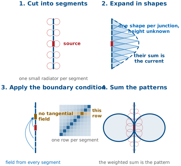
The same nine-segment dipole carries through all four panels. In the first, the wire is cut into segments and each segment is a small radiator whose pattern we already know from Lesson 6. In the second, the current is written as a sum of known shapes, one triangle per junction, and only their heights are unknown; the dashed line is the current they add up to. In the third, the boundary condition of a perfect conductor, no tangential electric field on the metal, is applied to one chosen segment: the fields that all the segments put there, together with the source field, must total zero. That is one row of the matrix: one row per segment, strongest on the diagonal because a segment feels itself most. In the fourth, the segment patterns, now weighted, add up to the pattern of the whole antenna.

It sounds simple, but there are consequences to this approach: every number the simulator reports inherits the choices in the model. The segments set how finely the current can vary, the basis functions set what shape it can take between the samples, the radius sets whether the thin-wire model describes the conductor at all, and the source sets the one segment the impedance is read from. The program checks none of them.

NEC — Numerical Electromagnetics Code, written at Lawrence Livermore in the 1970s and still the workhorse of wire-antenna modeling — is this method specialized to thin wires. It has no interface of its own: it reads a text file of cards and writes a text file of results, and every front end writes the same cards. Ours is nec_lab, written for this course and served from the course site; 4nec2 is the free Windows front end you will meet in the field. The cards do not move between versions the way menu items do, so the cards are what we teach.

NEC does not know about antennas. It knows about thin wires: straight segments with a length, a radius, and a position. A dipole is one wire with a segment count, and a Yagi is several wires. That simplicity makes NEC fast, but we have to follow some rules to avoid divergent results.

NEC drives one segment with a 1 V source, and that segment is the antenna terminal: there is no connector, no coaxial gap, and no balun in the model. The solve returns a whole vector of currents, one per segment, but the terminal impedance comes from exactly one entry in that vector. You applied a known voltage to the source segment, and the solver reports the current that flows there, so Ohm’s law finishes the job:

With the customary \(V_{\text{feed}} = 1\ \text{V}\) excitation, the input impedance is simply the reciprocal of the feed-segment current, and its complex character carries straight through: a feed current lagging the applied voltage gives a positive reactance, which means an inductive terminal.

There are three consequences to this approach. First, the impedance of the entire antenna comes from a single number in the solution, so it inherits whatever error that one segment carries. Second, the rest of the current distribution does not enter the terminal impedance at all; it sets the radiation pattern through the radiation integral. Third, those two facts together explain a failure mode you will meet later in the lab: a source placed on the wrong segment corrupts the impedance badly while barely moving the pattern, because the pattern is an integral over a current distribution that hardly changed.

Here \(\Delta\) is the segment length and \(a\) the wire radius. The first rule resolves the curvature of the current, and the pattern is an integral over that current, so a coarse mesh smears the pattern and the gain with it. The second keeps the phase nearly constant across a segment, which the basis functions assume; break it and the impedance drifts as you change the segmentation. The third is the thin-wire model’s own limit. It treats each segment’s current as a filament on the wire’s axis and evaluates its field on the surface, a distance \(a\) away, and that describes a segment only when the segment is much longer than the radius. When \(\Delta\) falls below about \(8a\) the segment is closer to a ring than to a piece of a line, the filament no longer describes it, and the matrix entries between neighboring segments become inaccurate.

The fourth rule is about the wire, not the segments. NEC models a wire as a single filament of axial current and enforces the boundary condition on the surface at radius \(a\). That is the problem it solves. The problem we want solved is a conducting cylinder, whose surface current can vary around the circumference and can have a component around the wire near the ends. The two problems have the same answer only when the circumference is small compared with a wavelength, \(2\pi a \ll \lambda\), because then nothing can vary around the wire within a wavelength and the surface current is the same as a filament on the axis. For a large-radius conductor NEC still returns a number, and it is the number for the filament, not for your antenna. The fifth rule is bookkeeping: an odd count puts a segment at the center, and the source card names a segment, so an even count lands the source half a segment off the feed.

Notice that two of these rules pull against each other, because refining the mesh drives \(\Delta\) down toward \(8a\). On a wire whose radius is large relative to the segment length you eventually run out of room, and that limit is informative rather than annoying: the segments have reached the length the thin-wire model needs, and refining further describes your antenna worse, not better.

The simulator does not report that it is wrong, so these four checks are the questions you have to ask it. Most groups meet at least two of these symptoms in a lab period, and the last row is the subject of the next frame.

Ask NEC for a pattern over the full sphere and it will report the average power gain. For a lossless antenna in free space that number must be 1.000, because every watt delivered to the terminals has to leave as radiation. This is a conservation-of-energy audit on your model, and it costs one extra run.

Every route runs the same tool and gives the same answers. The page has a form at the left and a NEC input file at the bottom right: the form writes that file, and the file is what NEC runs.

Choose Dipole in the antenna picker and press Build & solve, and the full deck is what appears. Read it before you read the plots, and type it out once by hand into the editor to prove you can:

CM ECE 444 L8 -- half-wave dipole, 915 MHz
CE
GW 1 21 0 0 -0.08197 0 0 0.08197 0.0005
GE 0
EX 0 1 11 0 1 0
FR 0 1 0 0 915 0
RP 0 181 1 1000 0 0 1 0
EN

CM and CE open the comment block, GE 0 closes the geometry in free space, and EN ends the deck.

All coordinates are in meters. The wire lies along \(z\), matching the course convention, so broadside is \(\theta = 90^\circ\) and the pattern cut above is the E-plane.

That is the whole point of the segmentation rules: you are the check. The tool can tell you that a number looks wrong; it cannot tell you that a model describes the antenna you meant to build.

A prediction written after the fact teaches you nothing, so step 1 is not optional and it is not a formality. Your reference numbers should not change once you see the simulated values.

That request sweeps \(\theta\) from 0° to 180° in 10° steps and \(\phi\) from 0° to 350° in 10° steps, and the final digit of the fourth field is what asks for the average gain. Record the value — it is a deliverable, and it is the one number that licenses all the others.

A wire cut to \(\lambda/2\) at 915 MHz will not resonate at 915 MHz, so determine where it does and by how much it misses. Then record the resonant length as a fraction of \(\lambda\) and the resistance there, keeping the segment count odd throughout and rechecking \(\Delta\) against \(8a\) after each change.

Record the peak gain, the E-plane HPBW, and the depth of the nulls along the wire axis, and confirm the H-plane cut is a circle to within a small fraction of a decibel. In the convergence study, identify both the point where the answer stops moving and the point where the \(\Delta > 8a\) rule begins to bite.

The pattern file drops straight onto your measured cut in Lesson 11, on one plot: the chamber dashboard’s Simulation section imports it and overlays it on the live cut. It is absolute dBi, and a chamber measures raw \(S_{21}\), so comparing the two means normalizing each to its own peak — which the dashboard does by default — and what that compares is shape. Comparing absolute levels is a gain-transfer measurement against a standard-gain horn, Lesson 9’s material, not something a file can fix. Save it somewhere you will find it in three lessons’ time.

Today’s dipole is the rehearsal. The product of this lab is the Analysis section of the midterm project: the simulated prediction for the antenna you will put on the range in Lessons 10 and 11. The project handout governs what that section must contain; this is how to build it.

1. Pattern. Predict the E-plane and H-plane cuts, and read the half-power beamwidth, the sidelobe level, and the gain from them.

2. Impedance. Predict \(Z_{\text{in}}\) and VSWR across the band you will measure, and the resonant frequency.

3. Checks. Run the average-gain test before recording anything, and show a convergence table so the reader knows the numbers have stopped moving.

4. Comparison. Set the simulation beside your hand analysis and account for every difference. “Simulation error” is not an account of anything, so name the mechanism. When the measurement comes in at Lesson 11 you will add a third column.

Build it the way you built the dipole today: predict by hand first, model the antenna, check the model, then compare. The dipole comparison table below, filled in, is the worked example.

Four of those rows should land within a few percent. The first row will not, so the mechanism behind it is worth stating here rather than leaving you to discover it by accident.

The number \(73 + j42.5\ \Omega\) is the impedance of the assumed sinusoid at exactly \(\lambda/2\), not of the wire. The solved current differs from the sinusoid near the tips and at the feed, and the impedance is read at the feed, where that difference is largest, so the resistance comes out near \(86\ \Omega\). Both models agree on where the wire resonates: the sinusoid at about \(0.476\lambda\) for this radius, which is where Lesson 7’s reactance curve crosses zero, and the solved current at about \(0.473\lambda\). A wire cut to exactly \(\lambda/2\) is therefore about 5% long under either model, which is why both call it inductive. The extra \(13\ \Omega\) of resistance comes from the difference in current shape, not from a difference in length; it is the same gap Lesson 7 noted between the model’s \(63\ \Omega\) and a real dipole’s \(70\ \Omega\) at resonance, and trimming does not remove it.

The difference in current shape has a name, the end effect. The assumed sinusoid goes to zero at the wire tips with a clean slope, while the real current approaches the tips more gradually because charge accumulates there. That larger current near the tips is visible in the convergence widget, and it is what raises the resistance and moves resonance slightly shorter.

The dipole you modeled today is the antenna you will hang on the analyzer next week, so keep your predicted impedance and resonant length where you can find them. Lesson 9 also introduces the midterm project, a pattern measurement on a dipole due 2 Oct — the measurement block runs early for that reason.