L29 - Range-Doppler and MTI#
Range-Doppler and MTI
A burst of 256 chirps measures velocity to 0.12 m/s, and a pulse canceller removes every return that does not move.
Lesson 29 · Antennas, Phased Arrays, and Radar Systems · Dr. Neil Rogers
Printing
To print the slides, switch to present mode and print: one slide a sheet, with room for notes. Print from read mode for the whole lesson.
Learning Objectives
- I can process FMCW radar data to produce range, range-waterfall, and range-Doppler results.
- I can apply moving target indication (MTI) processing to distinguish moving targets from clutter.
Lesson 26 defined the Doppler shift and the velocity resolution of a burst of pulses, Lesson 27 showed that adding the chirps of a burst coherently is what makes a weak target detectable, and Lesson 28 turned one chirp into a range profile. This lesson puts the three together. We send a burst of chirps, arrange the samples as a matrix, and take a second FFT across the chirps, which gives the range-Doppler map: every target at its range and its radial velocity at once. Then we remove the returns that do not move, the walls, the bench, and the kit’s own leakage, with moving target indication (MTI).
You will run all of this on your own kit in the L29 Lab, outside class, so the lesson carries the whole argument in read mode. We write the processing in terms of the two functions the course’s radar_lab.py provides for it, range_doppler and mti, which build on the L28 range code.
From One Chirp to a Burst
One chirp gives a range profile (L28).
A hand at 1 m/s moves 0.3 mm during a 300 µs chirp, 1% of a wavelength.
Velocity comes from comparing chirps: the burst sends 256, one every 0.5 ms.
In Lesson 28 one chirp gave one range profile. The echo, compared with the chirp still going out, is a tone whose frequency is proportional to range, and the range FFT sorts the echoes into range cells. The burst the L29–L31 Labs use sweeps 500 MHz in 300 µs, so the beat rises by 11.1 kHz for every meter of range, and the 0.30 m range cells of \(\Delta R = c/2B\) are 3.33 kHz apart.
A moving target also shifts the echo by its Doppler frequency, \(f_D = 2v/\lambda\), which is 66.7 Hz for every meter per second at the 3.0 cm wavelength of a 10 GHz carrier. Within a single chirp that shift is invisible. A hand moving at 1 m/s shifts the beat by 66.7 Hz, a fiftieth of one range cell, and moves only 0.3 mm while the chirp lasts. By the rule of Lesson 26, an observation 300 µs long resolves frequencies 3.33 kHz apart, which is 50 m/s of velocity.
To measure velocity we have to watch the target for longer, and an FMCW radar does it by repeating the chirp. The burst sends \(M = 256\) chirps of 300 µs at a pulse repetition interval (PRI) of 0.5 ms, so it watches every range cell for 128 ms. The rest of the lesson is how the radar turns those 256 range profiles into a velocity, following ADI’s Range Doppler Radar Processing lab.
Chirp Synchronization
Velocity compares the phase from chirp to chirp.
A 1 m/s hand moves the phase 12° a chirp, and a 1 µs start error moves it 42°.
The kit starts each chirp a fixed delay after the capture starts.
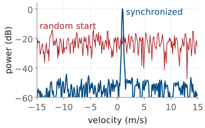
The range FFT of Lesson 28 needs only the frequency of the beat, so it does not care when the chirp started. The velocity measurement does. It compares the phase of the beat in one chirp with its phase in the next, and a moving target changes that phase by only a small, steady amount from chirp to chirp. A hand closing at 1 m/s moves 0.5 mm in one PRI, which shortens the round trip by 1.0 mm, a thirtieth of a wavelength, and advances the phase by 12°.
The beat phase also depends on when the samples start. A hand at 1.5 m has a beat of 117 kHz, the 0 m frequency of about 100 kHz that the L28 calibration measures plus 11.1 kHz per meter, so starting the samples 1 µs late changes the phase by \(360° \times 0.117 = 42°\). If the start time wanders by a microsecond from chirp to chirp, the error is larger than the signal we are trying to measure.
By default the board’s receiver simply fills a buffer with samples, with no relation between the start of the buffer and the start of any chirp. ADI’s Synchronizing Radar Chirps lab describes how the PHASER fixes this: a timing engine in the radio starts the capture and then fires each chirp at a programmed delay after it, one every PRI, so every chirp’s samples begin at the same point of its ramp. The capture format records that PRI as PRI, and every velocity on this page depends on it being exact.
The figure shows the difference in the hand’s range cell. With the chirps synchronized, the Doppler FFT of the next frames collects the hand into one sharp peak at +1 m/s. With each chirp starting at a random time within its PRI, the phase from chirp to chirp is random, and the same energy spreads evenly across every velocity: the hand is still there in range, but it has no velocity, and it sits 20 dB lower, close to the noise.
Fast Time and Slow Time
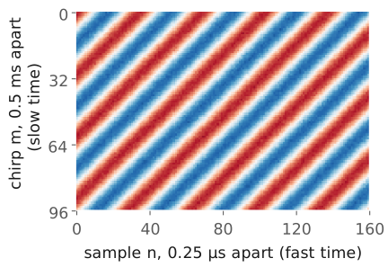
A row is one chirp: 1200 samples, 0.25 µs apart (fast time).
A column is one sample across chirps, 0.5 ms apart (slow time).
iqin your capture is this matrix,n_chirps × n_samples.
Stack the 256 chirps of a burst as the rows of a matrix. Along a row the samples are 0.25 µs apart, the 4 MSPS sample rate, and a row covers the 300 µs ramp in 1200 samples. That direction is fast time. Down a column the samples are one PRI apart, 0.5 ms, the same instant of each chirp; that direction is slow time. ADI draws the matrix the other way, chirps as columns; the capture format of the L28–L31 Labs stores it as the iq array, one row per chirp, n_chirps × n_samples, so the code on this page follows that layout.
The figure is the real part of that matrix for a single hand at 1.5 m, closing at 1 m/s, for the first 96 chirps and 160 samples. Across a row the beat oscillates at 117 kHz, one cycle every 34 samples; that frequency sets the range. Down a column the same sample oscillates once every 30 chirps, because the phase advances 12° a chirp; that rate measures the velocity. The stripes are diagonal because both are happening at once. A stationary target would draw vertical stripes, the same in every row.
The Phase From Chirp to Chirp
In slow time each range cell holds a tone at \(f_D = 2v/\lambda\).
At 1 m/s, \(f_D\) is 66.7 Hz and the phase advances 12° a chirp.
Take the range FFT of every row. The target now sits in the same range cell of every chirp, and that cell holds a complex number whose phase is the phase of the echo, \(-4\pi R_m/\lambda\), set by the round trip \(2R_m\) in wavelengths. Between chirps the target moves. With a closing speed \(v\), the range at chirp \(m\) is \(R_m = R_0 - v\ m\ T_\text{PRI}\), and substituting it gives the chain on the slide. The first term is a constant. The second grows linearly with \(m\), which is a tone in slow time at
the Doppler shift of Lesson 26, with the same sign: a closing target has a positive frequency. At \(\lambda = 3.0\) cm, 1 m/s gives 66.7 Hz, and in one PRI of 0.5 ms the phase advances \(360° \times 66.7 \times 0.5 \times 10^{-3} = 12°\).
Two effects that the chain leaves out are small for this burst. The Doppler shift also moves the beat in fast time, but at the ±15 m/s limit of the next frames it is 1.0 kHz against 11.1 kHz per meter, a range error of 0.09 m, under a third of a range cell. And the target moves during the burst: at 1 m/s it covers 0.128 m in 128 ms, less than one 0.30 m cell, which is the dwell limit of Lesson 27. A much faster target moves across several cells during the burst and smears in range; the widget later in the lesson shows it.
The Range-Doppler Map
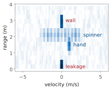
The radar takes a range FFT along each row, then a Doppler FFT down each column.
Returns that do not move sit in the 0 m/s column.
A spinner’s arms spread over ±2.2 m/s at one range.
The second FFT, down each column of the range-transformed matrix, finds the slow-time tone in every range cell. The result is the range-Doppler map: range on one axis, radial velocity on the other, and the power of each cell. Each FFT is the coherent integration of Lesson 27, so a target’s energy from all 1200 × 256 samples collects into one cell.
The figure is a map computed with the course’s burst numbers for a scene like the one in the L29 Lab. The kit’s own transmit leakage appears at 0 m and a wall at 3.0 m; neither moves, so both sit in the 0 m/s column, and they are the strongest returns on the map. A hand at 1.5 m closing at 1.0 m/s sits at +1.0 m/s. A fidget spinner at 2.1 m, three arms 3.5 cm long at 10 revolutions a second, has arm tips moving at \(2\pi \times 0.035 \times 10 = 2.2\) m/s; the arms move toward and away from the radar as they turn, so the spinner covers a band of velocities from −2.2 to +2.2 m/s at a single range. That spread is micro-Doppler, which Lesson 31 uses to classify targets.
Both FFTs use a Hann window, as the range FFT did in L28. The window matters more in Doppler than in range: the wall is 18 dB stronger than the hand here, and the first sidelobe of an unwindowed FFT is only 13 dB down, so without the window the wall’s sidelobes would spread across every velocity at its range. The Hann window puts the first sidelobe 31 dB down.
The provided radar_lab.py does this, and the L29 notebook runs it on your captures. The range FFT on each row is the one from L28.
def range_doppler(cap, window="hann"):
    """Range-Doppler map: (rd_db, range_m, vel_mps), rd_db indexed [range, velocity]."""
    rp = range_fft(cap, window)                 # n_chirps x n_bins, from L28
    r = range_axis(cap)
    keep = r >= 0
    rp = rp[:, keep]
    m = rp.shape[0]
    wd = _window(window, m)
    rd = np.fft.fftshift(np.fft.fft(rp * wd[:, None], axis=0), axes=0) / wd.sum()
    lam = C / cap["fc"]
    vel = np.fft.fftshift(np.fft.fftfreq(m, cap["PRI"])) * lam / 2
    rd_db = 20 * np.log10(np.abs(rd.T) + 1e-12)
    return rd_db, r[keep], vel
The velocity axis converts each Doppler bin to velocity with \(v = f_D\lambda/2\). The module follows the conventions of this page: positive velocity is closing, toward the kit, as in Lesson 26; the map is indexed [range, velocity], which is the order Lesson 30’s cfar_2d expects; only ranges at or beyond 0 m are kept; and range_doppler divides each FFT by the sum of its window, so a tone of amplitude 1 reads 0 dBFS whatever the window. A hand moving toward the kit therefore lands at positive velocity, and checking that on your own map is the first test of the velocity axis.
The Velocity Axis
With 256 chirps 0.5 ms apart, \(\Delta v = 0.12\) m/s and \(v_\text{max} = \pm 15\) m/s.
A target at +22 m/s appears at −8 m/s.
The Doppler FFT of \(M\) slow-time samples, \(T_\text{PRI}\) apart, has bins \(1/(M\ T_\text{PRI})\) apart in frequency, which is the rule of Lesson 26: watching for \(M\ T_\text{PRI}\) resolves its reciprocal. Converting with \(v = f_D\lambda/2\) gives the velocity resolution
The slow-time samples come once per PRI, so the Doppler FFT sees the tone sampled at the PRF, 2 kHz, and it can only tell apart frequencies within ±1 kHz. That is the maximum unambiguous velocity,
A faster target aliases. At +22 m/s the phase advances 264° a chirp, which the FFT cannot tell from −96°, so the map reports \(22 - 30 = -8\) m/s. These are the same two formulas ADI’s Range_Doppler_Processing.py prints as its velocity resolution and maximum velocity.
Choosing the Burst
Burst |
\(\Delta v\) (m/s) |
\(v_\text{max}\) (m/s) |
\(\Delta R\) (m) |
|---|---|---|---|
256 chirps, 500 MHz |
0.12 |
±15 |
0.30 |
32 chirps |
0.94 |
±15 |
0.30 |
200 MHz chirp |
0.12 |
±15 |
0.75 |
The chirp count sets \(\Delta v\), the bandwidth sets \(\Delta R\), and the PRI sets \(v_\text{max}\).
Each parameter of the burst controls one axis of the map. The number of chirps \(M\) sets the velocity resolution and nothing else: 32 chirps watch for 16 ms and resolve 0.94 m/s, 128 chirps resolve 0.23 m/s, and 256 chirps resolve 0.12 m/s. The chirp bandwidth sets the range resolution and nothing else: dropping from 500 MHz to 200 MHz widens every target from 0.30 m to 0.75 m in range. The PRI sets the velocity limit, and a longer chirp needs a longer PRI to fit in, so a 500 µs ramp, which cannot fit in a 0.5 ms PRI with time to reset, forces a slower PRF and a smaller \(v_\text{max}\). These are the experiments ADI’s range-Doppler lab suggests, and the L29 Lab runs the first two on your own kit.
More chirps also have two drawbacks. The integration gain of Lesson 27 is \(10\log_{10}M\): 24.1 dB for 256 chirps and 15.1 dB for 32, so a short burst has a higher noise floor on the map. A long burst refreshes the map less often, 128 ms for 256 chirps, and lets a fast target cross range cells while the burst lasts.
Range-Doppler Explorer
The widget computes a range-Doppler map from a simulated burst with the course’s numbers: leakage at 0 m, a wall at 3.0 m, and a hand at 1.5 m whose closing speed you set. Beside the map is the power gain of the MTI filter against velocity, with the hand’s speed marked; the next frames derive it. Start with the hand at +1 m/s and change the number of chirps: the hand’s spot narrows in velocity as \(M\) grows and the noise floor drops. Move the hand past +15 m/s and watch it reappear at negative velocity, and at more than a few meters per second watch it smear in range as it crosses cells during the burst. Turn chirp sync off: every target keeps its range and loses its velocity. Then step through the MTI settings at a few speeds.
Clutter at Zero Velocity
Leakage, walls, and the bench return the same phase every chirp.
They land in the 0 m/s column, up to 30 dB above a hand.
Their sidelobes and spread can cover a slow mover.
Everything that does not move returns the same echo on every chirp: the leakage from the transmit antenna straight into the receiver, the walls, the bench, the stand the kit sits on. Radar engineers call these returns clutter. On the map they all sit at 0 m/s, and in a lab room they are by far the strongest returns. In the scene of the earlier figure the leakage is 30 dB above the hand and the wall is 18 dB above it.
The Doppler FFT already separates clutter from a moving target, but removing the clutter still helps, for three reasons. A strong return has sidelobes in Doppler even with a window, and anything that changes the clutter slightly from chirp to chirp, a vibrating stand, a fan’s air moving a cable, the small timing error that chirp sync cannot remove, spreads its energy across nearby velocities, where a slow target competes with it. The CFAR detector of Lesson 30 estimates the noise from the cells around each test cell, and a clutter ridge in those cells raises the threshold for the targets beside it. And the spectrogram of one range bin, which the L29 Lab keeps for Lesson 31, has far less Doppler resolution than the full burst, so a strong clutter line there covers a wide band. Removing clutter before the Doppler FFT addresses all three, and that is moving target indication (MTI).
Pulse Cancellers
The top line is the 2-pulse canceller, and the bottom line is the 3-pulse.
A return that repeats exactly from chirp to chirp subtracts to zero.
The 3-pulse canceller is the 2-pulse canceller applied twice.
The simplest MTI filter subtracts each chirp from the one before it, sample by sample. ADI’s MTI Radar Processing lab calls it the two-pulse canceller. A return that is identical in two consecutive chirps, which is what a stationary return is when the chirps are synchronized, subtracts to zero. A moving target’s phase has advanced between the chirps, so the difference is not zero, and the target survives.
Applying the same subtraction to the output a second time gives
the three-pulse canceller. Its notch at 0 m/s is deeper and wider, as the next frame shows.
Both filters work across chirps, so we can apply them to the raw beat samples before the range FFT, as ADI’s script does, or to the range-transformed rows after it; the FFT is linear, so the two give the same map. Each output has one or two fewer chirps than the input. The provided radar_lab.py does this too, and the L29 notebook runs it on your captures. It returns a capture, so range_doppler(mti(cap, "2pulse")) works without any other change:
def mti(cap, kind="2pulse"):
    """A pulse canceller across chirps; returns a capture, one or two chirps shorter."""
    def cancel(x):                              # chirps on the second-to-last axis
        if kind == "2pulse":
            return x[..., 1:, :] - x[..., :-1, :]
        if kind == "3pulse":
            return x[..., 2:, :] - 2 * x[..., 1:-1, :] + x[..., :-2, :]
        if kind == "none":
            return x
        raise ValueError(f"kind must be '2pulse', '3pulse', or 'none', not {kind!r}")
    out = {**cap, "iq": cancel(cap["iq"])}
    if "iq_ch" in cap:
        out["iq_ch"] = cancel(cap["iq_ch"])
    return out
Canceller Response and Blind Speeds
Both null 0 m/s and every 30 m/s.
They peak at ±15 m/s, at +6.0 dB and +12.0 dB.
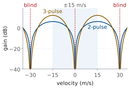
To find what the canceller does to a target of any speed, feed it the slow-time tone of the earlier frame,
The two-pulse output is
so the tone comes out with its power multiplied by
The three-pulse canceller is two of these in a row, so its power gain is the square,
Both gains are zero at \(f_D = 0\), the clutter. Both peak at \(f_D = \pm 1/(2T_\text{PRI})\), the edge of the unambiguous window at ±15 m/s, at 4 (+6.0 dB) and 16 (+12.0 dB).
The gain is also zero wherever \(f_D T_\text{PRI}\) is a whole number \(k\): the target’s phase then advances a whole number of turns from one chirp to the next, and the canceller cannot tell it from a stationary return. Those are the blind speeds,
every 30 m/s for this burst. The first blind speed is twice \(v_\text{max}\), which follows from the aliasing of the velocity-axis frame seen from the other side: a target at 30 m/s aliases to 0 m/s on the map, and the canceller removes it with the clutter. Nothing in the L29 Lab moves that fast, but a car or a drone can, and a radar that must see them changes its PRI from burst to burst so that a target blind at one PRI is visible at the next.
What MTI Removes
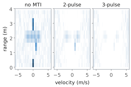
The leakage and the wall are gone.
A 1 m/s hand drops 13.6 dB (2-pulse) or 27.2 dB (3-pulse), and so does the noise in its velocity cell.
A target that stops, or crosses the beam, vanishes too.
The figure runs the scene of the range-Doppler frame through each canceller and draws all three maps on one scale. Both cancellers remove the leakage and the wall completely; what is left at 0 m/s is the residue of the small chirp-to-chirp timing error in the simulation, which is why chirp sync sets how deep the cancellation can go.
The cancellers also weaken moving targets, and they weaken the slow ones most. A hand at 1.0 m/s has \(f_D T_\text{PRI} = 66.7 \times 0.5 \times 10^{-3} = 0.033\), deep in the notch: the two-pulse canceller multiplies its power by \(4\sin^2(0.105) = 0.044\), −13.6 dB, and the three-pulse by −27.2 dB. The noise goes through the same filter. Each output adds independent noise samples, so the total noise power rises by the sum of the squared taps: \(1^2 + 1^2 = 2\), +3.0 dB, for the two-pulse canceller and \(1^2 + 2^2 + 1^2 = 6\), +7.8 dB, for the three-pulse. Against that total the hand’s SNR falls by 16.6 dB and 35.0 dB, and every target slower than about 7.5 m/s (two-pulse) or 8.6 m/s (three-pulse) loses SNR; that is the loss a detector would see if it looked at the canceled chirps without a Doppler FFT. The map does not compare the hand with the total. The Doppler FFT gives each velocity its own cell, and the noise in the hand’s cell passed through the same notch as the hand, so it drops by the same 13.6 or 27.2 dB, and the hand stands as high above its own floor as it did without MTI. The floor rises only toward ±15 m/s, by up to 6.0 and 12.0 dB, so the canceller shapes the floor the way it shapes the targets, and the L29 Lab’s notebook measures both. MTI improves the ratio of a target to the clutter, not to the noise, so it helps where clutter, not noise, limits what the radar can see.
Two more consequences follow from the notch. The canceller removes a target that stops moving, and also one moving across the beam, whose radial velocity is zero. The spinner shows both effects at once: the arms moving fastest along the line of sight survive, and the canceller removes the parts of its spectrum near 0 m/s with the clutter. For a hovering drone, ADI’s MTI lab points out, the body disappears but the blades’ micro-Doppler remains, which is what Lesson 31 classifies.
The choice of canceller is therefore a choice about the scene. With strong clutter and fast targets the three-pulse canceller gives the cleanest map; for a slow hand the two-pulse canceller, or none, keeps more of the target. The L29 Lab measures both on the same captures.
L29 Lab: Range-Doppler and MTI
Read a hand’s velocity and sign, then a fidget spinner’s micro-Doppler.
Predict, then read, the cells at 64, 128, 256 chirps and 200 MHz.
Compare MTI off, 2-pulse, and 3-pulse: which returns go and which stay.
The L29 Lab runs this lesson on your own kit, GUI first. The Phaser app does the live work: its Range + Velocity preset sends the burst, its Range-Doppler view draws the map, its MTI switch and MTI Mode run the cancellers, and Save Capture writes each burst to your laptop. In that view you check the velocity axis with your hand, closing and then opening, and watch a fidget spinner spread into a band of velocities at one range. You read the cells at 256 chirps on the kit and at 128, 64, and 200 MHz from the notebook and a recorded burst, and you switch the canceller between off, 2-pulse, and 3-pulse with a wall and your hand in the beam. The lab ends in the course’s notebook, where you run the provided range_doppler and mti on the bursts you saved and change a line or two for each of three tasks. You work on your own and turn in one packet in three parts: Part 1, Pre-Lab, the predictions, before you go to the bench; Part 2, Measurements, from your kit and the notebook; and Part 3, Writeup, after it. I check the packet and return it with feedback. It is the second piece of scaffolding for your final report.
The procedure follows ADI’s range-Doppler and MTI labs, which wave a hand and a fidget spinner at the same burst. The lab’s numbers are the app’s preset, not the round values above: a 9.9 GHz carrier (\(\lambda\) = 3.03 cm), 500 MHz in 300 µs, 256 chirps every 0.5 ms, 2 MSPS (600 samples a chirp), and \(c = 3.00\times 10^8\) m/s. The carrier moves the lesson’s velocity numbers by 1%: a 0.118 m/s cell, ±15.2 m/s, and 66.0 Hz and 11.9° a chirp at 1 m/s. The sample rate changes nothing on the map, because the range cell is still \(c/2B\) = 0.30 m. Their chirp synchronization page describes how the kit starts every chirp at a known time.
Pre-Lab Predictions
Setting |
\(\Delta v\) (m/s) |
\(\Delta R\) (m) |
Floor |
|---|---|---|---|
256 chirps, 500 MHz |
0.12 |
0.30 |
reference |
128 chirps |
0.24 |
0.30 |
+3 dB |
64 chirps |
0.47 |
0.30 |
+6 dB |
200 MHz |
0.12 |
0.75 |
same |
The table is the core of Part 1, and every entry follows from the frame Choosing the Burst, at the preset’s 9.9 GHz. The velocity cell is \(\lambda/(2MT_\text{PRI})\), so halving the chirp count doubles it, and the range cell is \(c/2B\), so 200 MHz makes it 2.5 times taller. The floor column is the integration gain of Lesson 27: half the chirps add 3 dB less, while a target’s level stays where it was, because range_doppler divides each FFT by the sum of its window. A Hann window makes a target’s spot one to one and a half cells wide 3 dB down, so a spot’s width on the screen is the cell you read. Part 1 also predicts the hand’s Doppler and the cancellers’ gain at its speed, from the frame Canceller Response and Blind Speeds: at 1.0 m/s, 66.0 Hz and 11.9° a chirp, −13.7 dB through the 2-pulse canceller and −27.4 dB through the 3-pulse.
A Spinner’s Micro-Doppler
Edge-on, each arm swings through \(\pm v_\text{tip}\) along the line of sight, which spreads the echo into a band at one range.
Three identical arms repeat every \(1/(3f_\text{rev})\), which puts the spectrum in lines \(3f_\text{rev}\) apart.
A fidget spinner held edge-on, its plane of rotation along the line of sight, moves each of its arms toward the kit for half a turn and away for the other half. An arm on a circle of radius \(a\) turning at \(f_\text{rev}\) revolutions a second has a radial velocity of
so over a burst its echo covers every velocity between \(-v_\text{tip}\) and \(+v_\text{tip}\). The arm spends the longest near the extremes, where its radial velocity turns around, so the band is brightest at its edges. For arms 3 cm from the hub at 15 revolutions a second, \(v_\text{tip} = 2\pi(0.03)(15) = 2.83\) m/s, a band of ±187 Hz at 9.9 GHz. The hub, and the hand that holds it, do not move, and sit at 0 m/s.
The band is not smooth. Three identical arms make a pattern that repeats every third of a turn, and a signal that repeats every \(1/(3f_\text{rev})\) seconds has its spectrum in lines \(3f_\text{rev}\) apart: 45 Hz, or \(\lambda(45\ \text{Hz})/2 = 0.68\) m/s, so the 0.118 m/s cells of the 256-chirp map resolve them. The spacing gives the spin rate without a ruler, and the band’s edge gives it with one; the lab measures both. Held face-on, the spinner moves its arms across the beam, with no radial velocity, and the band collapses toward the 0 m/s column: a hand never holds it exactly face-on, so a line or two either side of 0 m/s remains. This is the micro-Doppler of Lesson 26, the parts of a target moving relative to its body, and Lesson 31 uses it to tell one kind of target from another.
Bench Rules
Stand clear of the beam for every static and MTI reading.
Move the hand along the line of sight, at array height.
Hold the spinner edge-on, about 0.5 m out.
The burst sees everything that moves in the beam, and you are the largest mover in the room. While you read the wall or the cancellers on a static scene, step behind the kit or well to one side, or your breathing and sway appear as a smear of slow velocities across your range. When you are the target, keep it simple: a flat hand, 0.5 to 1 m out, pushed straight toward the array and pulled straight back at a steady speed. Moving the hand across the beam gives it almost no radial velocity, and the map shows it near 0 m/s.
Use a wall, or the L28 plate standing on its own, about 2.5 m in front of the kit as the static target the cancellers remove. Hold the spinner by its hub at arm’s length with its plane of rotation horizontal or vertical and pointed at the kit, so the arms move toward and away from it. A spinner with metal weights in its arms reflects more than an all-plastic one. The transmit antenna stays on OUT2, connected before you power the kit, as in the L28 Lab. No step needs a corner reflector.
Results
Keep your bursts of the hand with the wall, the spinner, and the static scene.
Keep your notebook with its edits.
Keep your Table B to E readings beside Part 1.
The L30 Lab runs CFAR on range-Doppler maps of this burst, with and without MTI, so keep your bursts, the notebook, and radar_lab.py together in your Module 4 folder, with the file names written in your packet. For the final report, keep three results: the velocity cell you read at three chirp counts against \(\lambda/(2MT_\text{PRI})\), the spinner’s spin rate from its band and from its lines, and what each canceller removed and what it kept. The report asks you to explain how a burst of chirps becomes a velocity, and what MTI does to a scene, in your own words; the packet’s tables are the evidence, not the explanation.
Equipment and Setup
You need:
the ADALM-PHASER kit with its Raspberry Pi and Pluto attached, and its transmit antenna;
a fidget spinner, ideally one with metal weights in its arms, and a ruler;
a wall about 2.5 m in front of the kit, or the L28 plate standing on its own at that range, and a tape measure;
your laptop, on the kit’s network for the Phaser app, with the Module 4 folder of the L28 Lab and this lab’s bundle unzipped into it (the Notebook Setup frame).
The Phaser app’s FMCW mode does every live step. Its Range-Doppler view draws velocity across and range up, positive velocity closing as in Lesson 26. Hover over any cell to read its velocity, range, and level in dB. Below the plot, Peak Range, Peak Velocity, and Peak Magnitude read the strongest cell that moves: they skip the cells within 0.3 m/s of zero, so read a wall or the leakage by hovering. The map’s colors run from each frame’s own peak down Color Span (dB), so after MTI the strongest thing left fills the scale whatever its level; read levels by hovering, never by color. The app’s dB scale sits about 18 dB below the notebook’s dBFS on the same burst (it normalizes and windows differently), so compare a change in dB between the two, not a level.
With the kit powered off, connect the transmit antenna to OUT2.
Power the kit, wait for the Pi to boot, and on your laptop open the radar app at
http://phaser-NN.local:8081, with your kit’s number for NN. Choose the FMCW tab at the top.In the FMCW section of the settings, set Preset to Range + Velocity (500 MHz in 300 µs, 256 chirps every 0.5 ms, 9.9 GHz), leave MTI off, open the Range-Doppler view, and press Start.
Save Capture downloads the current burst as a course
.npznamedphaser_range_doppler_<date>-<time>.npz: 256 raw chirps, whatever the MTI setting, so the notebook applies the canceller itself. Leave Subarray Channels off; this lab needs only the summed array. Rename each file for what it holds, for examplehand_closing_mine.npz, move it into your Module 4 folder, and write its name in the packet.
No Hardware?
Note
If your kit will not produce a clean burst, every procedure works without
one. Open the Phaser app’s simulator in a browser,
livethisdream.github.io/phaser/radar:
the same radar app, with a Scene menu in its FMCW section and a pill
that reads Simulated. Two things replace the bench there. A Scene
moves simulated targets live on the Range + Velocity preset: hand waves
a hand at 0.6 m, corners holds three corners at 1, 2, and 3 m, and
static holds a still target at 1 m with movers at 3.5 and 7 m.
Load Recording plays one of the course’s recorded bursts through the
same views as if it were live, with the MTI switch working on it; each
procedure below names the file. The recordings are in the lab’s bundle,
L29_lab.zip, with the
notebook. They simulate the PHASER on the app’s preset, with a kit whose
0 m frequency is 101.4 kHz and a wall at 2.5 m. The simulation times the
chirps perfectly, so the cancellers remove the wall completely, which no
kit does. Say in your packet which bursts are recorded rather than your own.
L29_static.npz: the leakage and the wall, nothing moving, Procedures A and EL29_hand_closing.npz: a hand moving from 1.0 m toward the kit at 1.0 m/s, Procedures B, D, and E and the notebookL29_hand_opening.npz: a hand moving from 0.7 m away from the kit at 1.5 m/s, Procedure BL29_spinner.npz: a spinner edge-on at 0.5 m, three arms on a 3 cm radius at 15 rev/s, Procedure C and task (c)L29_spinner_faceon.npz: the same spinner turned face-on, Procedure CL29_hand_closing_B200.npz: the closing hand at 200 MHz, Procedure D, with or without a kitL29_hand_still.npz: a hand held still at 0.8 m, Procedure EL29_hand_across.npz: a hand moved side to side across the beam at 0.8 m, Procedure E
Procedure A: Calibrate
Press Calibrate… in the FMCW section, hold the plate against the array, wait for the strongest return to settle, and press Calibrate: the app writes your kit’s 0 m frequency into 0 m Beat (kHz). Or type your L28 Table A value into that box. Record \(f_0\) in Table A.
Step clear of the beam. The leakage sits in the first range cell, at 0 m/s: the cell nearest 0 m, 0.17 m on the recorded data. Hover over it and record its range and level.
Find the wall, or the plate at 2.5 m: a spot at 0 m/s, the brightest on the recorded map. Hover over it and record its range on the map and on the tape.
Press Save Capture for the static scene, still clear of the beam.
Without a kit, leave 0 m Beat (kHz) empty and Load Recording L29_static.npz: a recording uses its own 0 m frequency, 101.4 kHz, which the Logs tab prints when it loads.
Procedure B: A Hand
Write your Part 1 prediction of the hand’s Doppler in Table B first.
Stand to one side of the kit and hold a flat hand in the beam about 1 m from the array, at array height.
Push the hand straight toward the array at a steady pace, about half a meter in half a second, and watch its spot. Record its range, velocity, and the sign of the velocity in Table B from Peak Range and Peak Velocity. Repeat a few times; record a typical push.
Pull the hand straight away from the array and record the same.
Press Save Capture during a push, with the wall still in view. The burst lasts 128 ms, so start the push before you press it.
Without a kit, choose the hand Scene in the simulator and watch the spot swing between about +0.9 and −0.9 m/s as the hand waves; then Load Recording L29_hand_closing.npz and L29_hand_opening.npz for Table B’s numbers.
Procedure C: A Fidget Spinner
Measure the spinner’s arm radius \(a\), from the center of the hub to the center of a weight, and record it in Table C.
Spin it hard and hold it by the hub, edge-on to the kit, about 0.5 m from the array at array height.
Hover along the band’s row to read its range, the velocities of its two edges, and, where the lines within it are visible, their spacing. Record them in Table C, and press Save Capture while it is spinning fast.
Turn the spinner face-on to the kit and write in Table C what happens to the band.
Without a kit, Load Recording L29_spinner.npz, then L29_spinner_faceon.npz. The notebook’s spinner cell prints the band’s lines and their spacing for either file.
Procedure D: Chirp Count and Bandwidth
Copy your Part 1 predictions into Table D before you change anything. The app’s presets all send 256 chirps of 500 MHz, so the kit gives the first row and the notebook and a recorded burst give the rest.
With the Range + Velocity preset, push your hand as in Procedure B, and read the width of its spot in velocity, in cells and in m/s, by hovering across it.
The 128 and 64 rows come from your Procedure B burst: the notebook’s task (a) keeps its first 128 and then 64 chirps, as a shorter burst would, and prints the width and the floor.
For the 200 MHz row, Load Recording
L29_hand_closing_B200.npzand read the height of the hand’s spot in range by hovering; the notebook’s map cell prints its width in range. No preset sends a 200 MHz chirp, so this row is recorded for everyone.
Without a kit, Load Recording L29_hand_closing.npz for step 1 and run task (a) on it.
Procedure E: MTI
Write your Part 1 predictions in Table E first. Read every level here by hovering.
Step clear of the beam with MTI off. Read the level of the wall’s spot and of the noise near it.
Turn MTI on with MTI Mode at 2-pulse, then 3-pulse, and read the same at the wall’s range and 0 m/s. Write down whatever is left.
Come back with your hand, pushing as in Procedure B, and read its spot’s level with MTI off, 2-pulse, and 3-pulse.
Hold your hand still in the beam, about 0.8 m out, and read its spot’s level the same three ways; then move it side to side across the beam and do the same.
Turn MTI off.
Without a kit, Load Recording L29_static.npz for steps 1 and 2, L29_hand_closing.npz for step 3, and L29_hand_still.npz and L29_hand_across.npz for step 4, switching the canceller as each plays. The notebook’s last cell reads the same rows in dBFS.
Notebook Setup
Download the lab’s bundle, L29_lab.zip, and unzip it into the Module 4 folder you set up in the L28 Lab’s Notebook Setup, with the same Python and packages. It holds L29_range_doppler.ipynb, a fresh radar_lab.py, the data README, and all eight recorded bursts, which the notebook opens by default, so it runs as shipped before you change anything. Move the bursts you saved with Save Capture into the same folder. Start Jupyter in the folder with jupyter lab and open L29_range_doppler.ipynb.
Procedure F: Run the Notebook
Do this part after the bench, from your saved bursts, in about 30 to 45 minutes.
Open
L29_range_doppler.ipynb, setCAPTUREin the first code cell to your hand burst with the wall in view, and run the cells from the top. The map cell reads your hand’s range, velocity, and width in range, the wall’s range, and the leakage.Task (a): run the chirp-count cell with
M = 256, then change that one line toM = 128and toM = 64. Record the velocity cell, the hand’s width 3 dB down, its level, and the floor for each in Table F.Task (b): replace
H_DB = Nonewith the canceller’s predicted gain at the hand’s Doppler, in dB, and run the MTI cell withKIND = "2pulse"; then change it toKIND = "3pulse". Record the hand’s change againstH_DB, the wall’s drop, and the floor in two places.Task (c): set
SPINto your spinner burst and run the map cell, which prints the band’s lines; setR_SPINto the range of the band and run the spectrogram withN_WIN = 64, thenN_WIN = 32. Record the band’s edges, the Doppler cell, and the time between columns.Save the notebook with its edits and plots and upload the
.ipynbwith the packet.
Each task’s markdown cell states the result to check against. Anything you do beyond the three tasks belongs in your report’s Extra Effort.
Lab Packet
Summary
Symbol / idea |
What it is |
Number for the L29 burst |
|---|---|---|
Burst |
\(M\) chirps, one every \(T_\text{PRI}\) |
256 chirps of 300 µs, 0.5 ms PRI, 128 ms |
Chirp sync |
every chirp starts a fixed delay after the capture |
1 µs of error shifts the phase 42° at 117 kHz |
Fast time |
samples within one chirp, a row of |
1200 samples, 0.25 µs apart |
Slow time |
the same sample across chirps, a column |
256 samples, 0.5 ms apart |
Slow-time tone |
\(f_D = 2v/\lambda\) in every range cell |
66.7 Hz, 12° a chirp, at 1 m/s |
Range-Doppler map |
range FFT on rows, Doppler FFT on columns |
0.30 m by 0.12 m/s cells |
Velocity resolution |
\(\Delta v = \lambda/(2M\ T_\text{PRI})\) |
0.12 m/s; 0.94 m/s at 32 chirps |
Maximum velocity |
\(v_\text{max} = \pm\lambda/(4T_\text{PRI})\) |
±15 m/s; +22 m/s shows at −8 m/s |
2-pulse canceller |
\(y_m = x_m - x_{m-1}\), gain \(4\sin^2(\pi f_D T_\text{PRI})\) |
−13.6 dB at 1 m/s, +6.0 dB at 15 m/s |
3-pulse canceller |
\(y_m = x_m - 2x_{m-1} + x_{m-2}\), gain squared |
−27.2 dB at 1 m/s, +12.0 dB at 15 m/s |
Noise gain |
sum of the squared taps, averaged over velocity; the floor takes the canceller’s shape |
+3.0 dB and +7.8 dB |
Spinner, edge-on |
a band to \(\pm v_\text{tip} = \pm 2\pi a f_\text{rev}\), lines \(3f_\text{rev}\) apart |
±2.83 m/s and 0.68 m/s at 3 cm, 15 rev/s |
Blind speeds |
\(v_\text{blind} = k\lambda/(2T_\text{PRI})\) |
every 30 m/s |
The numbers are the lesson’s round 10 GHz, 4 MSPS values. The kit’s Range + Velocity preset, which the L29 Lab uses, is 9.9 GHz at 2 MSPS: 600 samples a chirp, 0.5 µs apart; 66.0 Hz and 11.9° a chirp at 1 m/s; 0.118 m/s cells; ±15.2 m/s; −13.7 and −27.4 dB through the cancellers at 1 m/s; and blind speeds every 30.3 m/s.
Looking Ahead
Lesson 30 takes the range-Doppler map this lesson produces and decides which cells hold targets, setting the threshold from the cells around each one rather than from a noise power assumed in advance, as Lesson 27 showed it must. The L30 Lab runs that detector on the maps you make in the L29 Lab, with and without MTI. Lesson 31 then looks inside a detection: the slow-time signal of one range cell, cut into short pieces and transformed one piece at a time, is a spectrogram, and the micro-Doppler in it, the spinner’s arms or a walker’s limbs, is what tells one kind of target from another.