In Lesson 18 we derived the steering law and used it to fill in a table of element phases for the PHASER’s eight-element array. The L18 Lab packet starts from that table: Part 1, the pre-lab you completed before class, redoes it at your HB100’s frequency, predicts the beamwidths, and sizes the error budget. Today you place the source at measured angles on a protractor arc, and also commands the peak to the same angles from the GUI, and records where the trace peaks, how wide it is, and what the GUI writes into Phase Control. Part 3, on your own before Lesson 19, reconciles those numbers with the predictions.

The array is fixed: \(N = 8\) elements, E1 to E8, on a \(d = 14\ \text{mm}\) pitch. The source is an HB100 Doppler module at a nominal 10.525 GHz, so \(\lambda = 28.5\ \text{mm}\) and \(d/\lambda = 0.491\), with \(c = 3.00\times 10^8\ \text{m/s}\). Steering to \(\theta_0\) takes a progressive phase of

Lesson 18 worked the same table at the workshop’s 10.3 GHz, where \(kd = 173.2^\circ\) and the 30° step is 86.6°. At 10.525 GHz the step is 88.4°, and Part 1 of the packet redoes the table at the frequency your kit reported in Lesson 17, because every phase in the lab depends on it.

The phase shifters produce a value between 0° and 360°, so element E\((n+1)\), which is element \(n\) in Lesson 18’s numbering, gets \(n\Delta\phi\) wrapped modulo 360°. Wrapping changes nothing physically at one frequency, because a phase shift of 360° is no phase shift at all. For \(\theta_0 = 30^\circ\) the eight values are these, and E6 through E8 are the ones that have wrapped:

Each entry is a multiple of the unrounded step, 88.41°.

The x-axis of the PHASER’s Rectangular plot is the angle the sweep steers to, not a measured arrival angle. With Lab Preset 1 loaded, the instrument steps the element-to-element phase one phase-shifter LSB, 2.8125°, at a time, and plots each step at the angle that phase steers to; the steps past endfire collect at ±90°, which is why the edges of the trace look crowded.

The trace is a picture of the pattern because of Lesson 18’s “The Steered Pattern”: the array factor depends only on \(\sin\theta - \sin\theta_0\), and its magnitude is even, so power received from a source at \(\theta_{\text{src}}\) as the beam steps across \(\theta_0\) traces the same curve as the pattern of a beam steered at the source. It peaks where the steered angle equals the source angle.

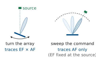
Rotating the array in front of a fixed source would record a different quantity. Turning the array moves the source across the element pattern as well, so the rotation records the element pattern times the array factor (Lesson 16). The sweep holds the element pattern fixed at the source’s direction, so it records the array factor alone, scaled by the element pattern’s value there. That scale factor is what a peak-level comparison between two source positions measures. Every point of the sweep also uses a different set of element phases, so the beamformer’s own errors, phase quantization and gain imbalance, shape the trace.

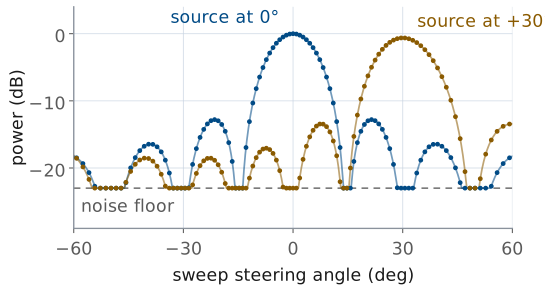
The bench puts the peak at the same angles two ways. In the physical run, Phase Control holds zero, the sweep’s own ramp is the only steering, and the trace peaks at the source’s angle on the arc. In the commanded run, the source stays at boresight and Apply in the Beam Steering section loads per-element offsets that shift the trace: Apply 30 puts a boresight source’s peak at +30°.

The two traces have the same width, because both shift the same function of \(\sin\theta - \sin\theta_0\) to the same place. Their peak levels differ. In the physical run the source sits 30° off each element’s own boresight, and the element pattern lowers the whole trace by its roll-off at 30°. In the commanded run the source never leaves the elements’ boresight, so the peak level matches the 0° trace. That difference is the measurement of scan loss (Lesson 18, “Scan Loss”).

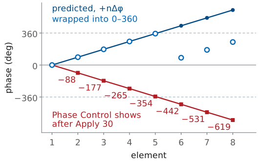
When you type 30 into Steer Angle (deg) and press Apply, the GUI computes \(\Delta\phi\) from the Signal Freq on screen and writes \(-n\Delta\phi\) into the Phase Control boxes, rounded to whole degrees and not wrapped. At 10.525 GHz the boxes read 0, −88, −177, −265, −354, −442, −531, and −619. The sliders beside the boxes stop at ±180°; read the boxes.

The minus sign is deliberate. During a sweep the backend adds its own ramp, \(+n\Delta\phi_s\), to whatever Phase Control holds, so element \(n\) carries \(n(\Delta\phi_s - \Delta\phi_0)\). A boresight source needs no ramp at all, so the array points at it where \(\Delta\phi_s = \Delta\phi_0\), which is the plotted angle +30°. Apply is therefore the offset that makes a boresight source look like a source at \(+\theta_0\) on the sweep plot. On their own, with no sweep ramp added, the offsets would point the beam to −30°. To compare the read-back with the wrapped ramp, reduce it modulo 360°: E6’s −442° is 278°, which is \(360^\circ - 82.0^\circ\).

The GUI computes \(\Delta\phi\) with \(c = 299792458\ \text{m/s}\), not the \(3.00\times 10^8\ \text{m/s}\) of our prediction, so one element can differ by 1° after rounding: our \(-n(88.41^\circ)\) gives −530 for E7, and the GUI’s \(-n(88.47^\circ)\) gives −531.

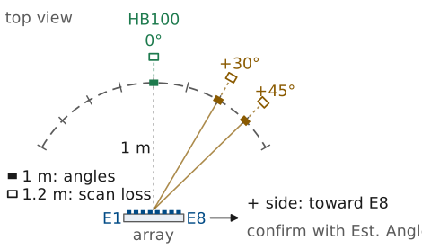
You need the ADALM-PHASER kit on its stand, connected to your laptop by the Ethernet cable as in Lesson 17; the HB100 on a tripod about 1 m from the array face, at the height of the patch row; and a protractor arc of 1 m radius centered under the middle of the array, between E4 and E5.

One meter is Lesson 17’s far-field distance for this array, \(2D^2/\lambda = 0.88\ \text{m}\) with \(D = Nd = 112\ \text{mm}\). Center the arc on the array, not on the board’s edge: an arc centered 10 mm off the middle of the array shifts the reference angle by about 0.5°. The arc serves the angle readings. The scan-loss levels need more distance, 1.2 m (4 ft) or more on the same three lines, for the reason given in Run 1.

Lesson 18’s sign convention puts \(+\theta\) on the E8 end of the array, the end the wave reaches first. Looking at the front of the array, the patch face, E1 is at the right end of the row and E8 at the left, as in the L17 Lab, so \(+\theta\) is to your left as you face the patches. In the figure, which looks down on the bench from above, that puts E8 on the right. Confirm the sign on your kit before you record anything: with the source on the \(+\) side, Angle reads positive.

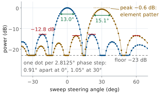
The calculated column comes from the array factor for \(N = 8\) at \(d/\lambda = 0.491\). The \(1/\cos\theta_0\) broadening of Lesson 18 gives \(12.9^\circ/\cos 30^\circ = 14.9^\circ\) from the rule’s broadside width, and the exact array factor gives 13.0°, 15.1°, and 18.7°. A sweep sampled about a degree apart reads each width to about a degree. dBc is dB relative to the main-lobe peak; the sweep’s floor sits about 23 dB below the peak, and the first sidelobes come up out of it at −11 to −13 dBc.

The peak drop is the element pattern’s roll-off, the scan loss of Lesson 18. Its ideal-element bound is

and −1.5 dB at 45°. A patch element rolls off faster, closer to \(\cos^{1.3}\theta\) to \(\cos^{1.5}\theta\) in power, so expect −0.8 to −0.9 dB at 30°; Lesson 21 derives the element pattern. These values hold with the source at 1.2 m or more, where my kit read −0.7 dB at 30°. At 1 m the same kit read only −0.2 to −0.4 dB, so a level taken that close comes out smaller than theory. The 45° drop is limited by reflections from the room: the kit read −1.0 dB there, less than the ideal bound, so treat that row as an estimate. The commanded run keeps the source on the elements’ boresight, so its peak does not drop. The peak-drop rows are hardware measurements: the simulator has no element pattern and reads 0.0 dB in both runs.

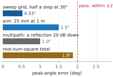
The measured peak angle will not equal the arc angle exactly, and the beamwidths will not equal 13.0° and 15.1° exactly. Three independent effects account for the difference, and Part 1 of the packet sized all three before the measurement.

Sweep grid. With Use Bits on, the sweep steps the element phase one 2.8125° LSB at a time. One step moves \(\sin\theta\) by \(2.8125^\circ/176.8^\circ = 0.0159\), which is 0.91° of angle at broadside and 1.05° at 30°, widening as \(1/\cos\theta\). The trace holds no information between samples, so a peak read off it can be wrong by half a step, 0.53° at 30°.

Arc placement and aim. At 1 m, one degree of arc is 17.5 mm, so a tripod placed by eye to within 25 mm gives a 1.4° error in the reference angle; centering the arc and pointing the module bring the budget figure to 1.5°. This error is in the reference, not in the array.

Multipath. The bench, the walls, and the people nearby return copies of the tone. A reflection 20 dB below the direct path has an amplitude ratio of 0.1, so, depending on its phase, it raises or lowers the level by

a ripple on the main lobe that moves the apparent peak by up to about a degree. Absorber behind the array and a clear arc both reduce it.

Because the three are independent, they combine as a root sum of squares:

A peak within ±2° of the reference meets the standard, and agreement to 0.1° would point to a mistake in the comparison rather than an unusually good measurement.

Lesson 19 and the fox hunt put today’s skill to work while it is fresh: the peak of the sweep is a bearing, and bearings from several stations cross at the source.

Today we compared measured beamwidths and sidelobes with values from Lesson 16’s closed form and Lesson 18’s broadening rule. Lesson 20 takes the closed form

and extracts every feature of the trace you just recorded from it: where the nulls fall, why the first sidelobe sits 12.8 dB down, how the beamwidth follows

and what changes when elements are switched off. Bring today’s traces to that lesson; the derivation is easier to trust with the measurement in front of you.