L16 - The Array Factor and Pattern Multiplication#
The Array Factor and Pattern Multiplication
The sum of the element phasors reduces to one compact expression, the array factor.
Lesson 16 · Antennas, Phased Arrays, and Radar Systems · Dr. Neil Rogers
Printing
To print the slides, switch to present mode and print: one slide a sheet, with room for notes. Print from read mode for the whole lesson.
Learning Objectives
- I can derive the array factor for an arbitrary linear array and apply pattern multiplication.
From Apertures to Elements
In Lesson 15’s continuous aperture, length set the beamwidth and taper set the sidelobes.
The PHASER has 8 patches in a row, not a continuous aperture.
Their phasor sum, the array factor, predicts every pattern this module measures.
Lesson 15 treated an aperture as a continuous sheet of current and read its beamwidth from the aperture length and its sidelobes from the taper. Now we replace that continuous aperture with \(N\) discrete elements on a line, each fed its own copy of the signal. The far fields still add as phasors, so the same reasoning applies, and the sum reduces to one compact expression, the array factor, which predicts every feature you will measure on the PHASER for the rest of this module.
Part 1: The Linear Array
The array has \(N\) identical elements spaced \(d\) apart, with weights \(a_n\).
Every element radiates the same pattern; only the weights and the positions differ.
We measure the scan angle \(\theta\) from broadside, as the PHASER GUI does.
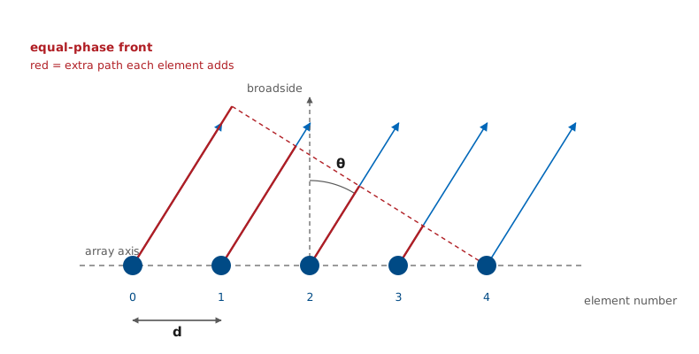
We put \(N\) identical elements on a straight line, spaced a distance \(d\) apart, and feed element \(n\) a copy of the same signal with complex weight \(a_n\). Every element radiates the same pattern; only the weights and the positions differ.
The Scan Angle
Module 3 measures \(\theta\) from broadside, as the PHASER GUI does.
Lesson 6’s \(k_z = k\cos\theta_{\text{polar}}\) becomes \(k\sin\theta\).
Broadside moves from \(\theta_{\text{polar}} = 90^\circ\) to \(\theta = 0\).
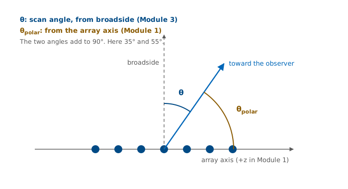
Module 3 measures the scan angle \(\theta\) from broadside, the direction perpendicular to the array face, with \(-90^\circ \le \theta \le +90^\circ\). Every PHASER plot, the GUI’s angle axis, and the phased-array literature use this convention.
Module 1 measured the polar angle from the \(+z\) axis for a line source lying on \(z\). The two are the same picture read from different reference directions, so the space frequency \(k_z = k\cos\theta_{\text{polar}}\) of Lesson 6 becomes \(k\sin\theta\) here. Broadside, which was \(\theta_{\text{polar}} = 90^\circ\), is now \(\theta = 0\). This is the only place in the course where we set the two conventions side by side; from here on \(\theta\) means the scan angle.
Extra Path Length and Phase
The far-field rays are parallel, so only the projection of \(nd\) onto the look direction matters.
\(\psi = kd\sin\theta\) is the inter-element phase, neighbor to neighbor: 0 at broadside, \(\pm kd\) at endfire.
Element \(n\) arrives carrying \(a_n\ e^{\ jn\psi}\).
A far-field observer sees the array from a single direction, so the rays leaving the elements are parallel. Element \(n\) sits \(nd\) farther along the array axis than element 0, and along a ray heading off at angle \(\theta\) that position shortens the path to the observer by \(\Delta r_n = n\ d\sin\theta\). The wavenumber \(k = 2\pi/\lambda\) converts distance to phase, so a path shorter by \(\Delta r_n\) is a phase lead of \(k\ \Delta r_n\), and element \(n\) arrives at the observer carrying
relative to element 0.
Every term carries the same step per element, \(kd\sin\theta\), so we give it a name: \(\psi = kd\sin\theta\) is the inter-element phase, the phase by which each element leads its neighbor as seen from direction \(\theta\). It is not the progressive phase \(\beta\) that the phase shifters apply, and not the ADAR1000’s 2.8125° phase step; it is what the observer sees, the geometry less any applied \(\beta\). It is the only way the angle enters the sum. Each direction gives one value of \(\psi\): broadside, \(\theta = 0\), gives \(\psi = 0\), where every element arrives in phase, and endfire, \(\theta = \pm 90^\circ\), gives the largest step, \(\psi = \pm kd\). For the PHASER, \(kd = 173^\circ\). The rest of the lesson works in \(\psi\) and converts back to \(\theta\) through this one relation.
The same path differences change the amplitude \(1/r\) by a negligible amount. The PHASER is 112 mm long, so its far field begins at \(2D^2/\lambda = 0.86\ \text{m}\) (Lesson 5). At a 30 m range, 112 mm of path changes \(1/r\) by less than 0.4%, but it spans 3.85 wavelengths, or nearly 1400° of phase. This is the parallel-ray approximation of Lesson 6: we keep the path difference in the phase and drop it from the amplitude.
Superposition
Identical elements share \(E_0(\theta)\), so it factors out and leaves the array factor: Lesson 6’s space factor \(S(\theta)\), with a sum in place of the integral.
Steering subtracts the progressive phase from \(\psi\): \(\psi = kd(\sin\theta - \sin\theta_0)\) (Lesson 18). Today \(\theta_0 = 0\).
The total far field is the sum of the element fields, and because every element has the same pattern, the common factor \(E_0(\theta)\ e^{-jkr}/r\) comes out in front of the sum. The array factor \(AF(\theta)\) is the sum that remains. It depends only on how many elements there are, where they sit, and what weights we feed them. It does not depend on the type of element.
The array factor is the discrete form of the space factor \(S(\theta)\) of Lessons 6 and 15. There the current, or the aperture field, was continuous, and \(S(\theta)\) was its integral weighted by \(e^{\ jkx\sin\theta}\). Here the current exists only at \(N\) points, so the integral becomes a sum over the elements. The normalized pattern \(\vert F(\theta)\vert\) is \(\vert E\vert\) divided by its peak, and the \(1/r\) and \(e^{-jkr}\) drop out of it, so \(\vert F\vert\) is the element’s own pattern times \(\vert AF\vert\). That is Lesson 6’s element factor times space factor, and Part 3 names the element’s part \(EF\).
The Array Factor From the Radiation Vector
Lesson 6 computed the far field of a \(z\)-directed current from its radiation vector,
An array is a current that exists only at the element positions. If we model element \(n\) as a point source of strength \(a_n\) at \(z' = nd\), the current is
and the integral picks out one term per element:
The last line is \(AF(\theta)\). The phasor sum and the radiation integral give the same result: the array factor is Lesson 6’s space factor for a current made of \(N\) point samples. A real element replaces each point source with its own pattern, which is the element factor.
Steering Phase
\(\beta = kd\sin\theta_0\) steers the beam to \(\theta_0\); Lesson 18 derives it.
Today \(\theta_0 = 0\), so \(\psi = kd\sin\theta\).
If the weights carry a progressive phase \(\beta\) per element, that phase adds to the geometric term, and both collect into the inter-element phase \(\psi\). The ramp \(\beta = kd\sin\theta_0\) steers the beam to \(\theta_0\), and Lesson 18 derives it. For the rest of today \(\theta_0 = 0\) and \(\psi = kd\sin\theta\), so every result below is the broadside case.
Key Point: A Sum of Phasors
The array factor is a sum of unit phasors, one per element, whose phases advance by \(\psi\) from element to element. Every feature of the pattern comes from how those phasors line up.
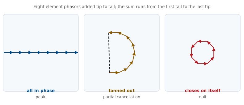
Read the three cases from left to right. At \(\psi = 0\) every phasor points the same way and the sum is \(N\), the largest it can be. As \(\psi\) grows the chain fans out and the sum shortens. When the fan has turned through a full circle, \(N\psi = 2\pi\), the chain closes on itself and the sum is exactly zero. That is the first null, and the closed form below locates it for every \(N\).
Phasor Chain Explorer
The left panel draws the \(N\) element phasors tip to tail, with each one turned \(\psi\) from the last, and the navy arrow is their sum. The widget references the phase to the array center, so the sum always lies along the horizontal axis and points left where the array factor is negative. The right panel is \(\vert AF\vert\) against scan angle, with a marker at the current \(\theta\). Start at broadside, where the chain is straight and the sum is \(N\). Drag \(\theta\) slowly: the chain curls, the sum shortens, and at 15.1°, where \(\psi = 45^\circ\) and \(N\psi = 360^\circ\), the chain closes into an octagon and the sum is zero. Keep going to 21.9° to find the first sidelobe, −12.8 dB, where the chain has wound about one and a half turns.
Part 2: Uniform Excitation
\(\vert e^{\ j(N-1)\psi/2}\vert = 1\): it is the phase of the array’s center, so \(\vert AF\vert\) never sees it.
Dividing by \(N\) sets the peak to 1.
Setting every weight to 1 turns the sum into a finite geometric series in \(e^{\ j\psi}\). To close it, we factor half of each exponent out of the numerator and the denominator, which leaves a difference of conjugate exponentials in each bracket. Euler’s formula turns each bracket into \(-2j\sin(\cdot)\), and the \(-2j\) factors cancel between top and bottom.
The leading factor \(e^{\ j(N-1)\psi/2}\) has magnitude 1, so it changes the phase of \(AF\) and never its size. It comes from where we put the phase reference. We measured every element’s phase from element 0, at one end of the array. The center of the array sits \((N-1)d/2\) from element 0, and \((N-1)\psi/2\) is exactly the phase that point carries. Pulling that phase out of every term counts each element from the center instead:
The centered sum pairs each element with its mirror image across the center, and each pair adds to \(e^{\ jm\psi} + e^{-jm\psi} = 2\cos(m\psi)\), so the sum is real: it is the ratio of sines. Measured from the center, the leading factor is simply absent. Measured from element 0, it is there, but the pattern is \(\vert AF\vert\) and \(\vert e^{\ j(N-1)\psi/2}\vert = 1\), so it drops out either way. Dividing by \(N\) then normalizes the peak to 1. The main lobe, the nulls, and the sidelobes all follow from this expression.
Main Lobe and Nulls
At \(\psi = 0\) the limit of \(0/0\) is 1, so the beam points at \(\theta_0\).
Nulls fall where the numerator vanishes and the denominator does not, \(m = 1, \ldots, N-1\).
The total length \(Nd\) sets the nulls, not \(d\) alone.
Main lobe. At \(\psi = 0\) both numerator and denominator vanish, and the limit is 1. The peak therefore sits where \(\sin\theta = \sin\theta_0\), which at broadside is \(\theta = 0\). The function is periodic in \(\psi\) with period \(2\pi\), so the peak repeats every \(2\pi\); Part 4 finds the spacing at which a repeat reaches a real angle.
Nulls. The numerator vanishes when \(N\psi/2 = m\pi\), and the denominator is nonzero as long as \(m\) is not a multiple of \(N\). The nulls depend on \(N\) and \(d\) only through the total length \(Nd\).
Sidelobes
There are \(N - 2\) sidelobes per period, one between each pair of nulls, and the first is the tallest.
The first peaks near \(N\psi/2 = 3\pi/2\), halfway between the first two nulls.
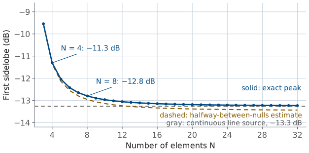
Between consecutive nulls the numerator swings back to ±1, so a sidelobe sits in each gap: \(N - 2\) of them across one period. Their heights fall off as \(1/\sin(\psi/2)\), so the tallest is the one nearest the main lobe. The numerator reaches its peak magnitude halfway between its first two zeros, at \(N\psi/2 = 3\pi/2\), and evaluating \(AF_N\) there gives \(2/(3\pi) = 0.212\) for large \(N\), or −13.5 dB.
The denominator is still growing across that gap, so the true peak sits slightly closer to the main lobe, where the denominator is smaller. Locating it exactly gives −13.3 dB, which is the uniform line-source number from Lesson 6. At \(N = 8\) the value is −12.8 dB. The figure plots the exact level against \(N\): a short array has a higher first sidelobe, and by \(N = 16\) the level is within 0.2 dB of the line source. The estimate runs a fraction of a decibel low at every \(N\), for the reason above. Uniform excitation leaves the first sidelobe about 13 dB below the peak in a discrete array, as it did in the continuous aperture of Lesson 15, and Lesson 22 lowers it with a taper.
Reading the Closed Form
Feature |
Uniform array |
|---|---|
Main-lobe peak |
\(\theta = \theta_0\) |
Null \(m\) |
\(\sin\theta_m = \sin\theta_0 + m\lambda/Nd\) |
First-null beamwidth |
\(2\arcsin(\lambda/Nd)\) at broadside |
Half-power beamwidth |
\(\approx 0.886\ \lambda/(Nd\cos\theta_0)\) |
First sidelobe |
−13 dB (−12.8 dB at \(N = 8\)) |
Sidelobe count |
\(N - 2\) per period |
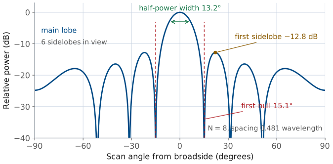
The figure marks the three features on the PHASER’s own array, \(N = 8\) and \(d/\lambda = 0.481\): a half-power width of 13.2°, a first null at 15.1°, and a first sidelobe at −12.8 dB, with six sidelobes, \(N - 2\), between the nulls.
The half-power row uses the line-source constant of Lessons 6 and 15 with \(L = Nd\), and Lesson 20 derives it for the array, along with the \(1/\cos\theta_0\) broadening under steering. The constant is close but not exact for a short array: the PHASER’s exact half-power width is 13.3°, against 13.2° from \(0.886\ \lambda/Nd\).
Part 3: Pattern Multiplication
It requires identical, identically oriented elements, so \(E_0(\theta)\) factors out of the sum.
In decibels the two patterns add.
This is Lesson 6’s element factor times space factor, with a sum in place of the integral.
Nothing in Part 1 required the elements to be isotropic. It required them to be identical and identically oriented, which let \(E_0(\theta)\) come out of the sum. That factoring is pattern multiplication.
The element factor \(EF\) is the pattern one element would produce by itself. The array factor \(AF\) is what the arrangement adds. Their product is the array’s pattern. In decibels the two curves add, which is why a log plot is the natural place to check the result.
This is the Lesson 6 split, pattern equals element factor times space factor, with the continuous space factor replaced by a discrete sum. The element factor comes from the physics of the radiator; the array factor accounts for where the elements sit and how we feed them.
From Two Patterns to One
This is Lesson 6’s two sources (“Two Sources in Space”), now with real elements and a wide spacing. The widget starts with two short dipoles \(4\lambda\) apart. Close to either one, its own \(1/r\) wave is much stronger than its partner’s, so the map shows that element’s own figure-eight. Farther out the two waves overlap and interfere, and the fringes on the map are the far-field lobes forming. They stop changing shape with distance only at the pair’s far-field distance, \(2D^2/\lambda = 32\lambda\) (Lesson 5), well off the map.
The far-field pattern obeys pattern multiplication at any spacing: the power is \(\vert EF\vert^2 \vert AF\vert^2\), with
Its peaks fall where \(\sin\theta = m\lambda/d\). At \(d = 4\lambda\) that gives \(m = 0, \pm 1, \ldots, \pm 4\), nine lobes 14.5° apart near broadside, with the outer pair shrunk by the dipole’s null along the array axis. The power of the sum is
and the cross term changes sign from each lobe to the next null. Averaged over one lobe spacing, about 15°, it cancels and leaves the amber curve, \(2\vert EF\vert^2\), which is what two independent antennas give, each radiating its own pattern.
Press “far apart” to move them \(10\lambda\) apart. The map widens, each figure-eight stands clear of the other near its own element, and the fringes between them grow faint. In the far field the lobes are now only 5.7° apart near broadside, too fine for a receiver with any spread in angle or frequency to follow, and their average is the same amber curve. Far enough apart, the pair behaves as two independent antennas.
Press \(\lambda/2\). Now \(\sin\theta = m\lambda/d\) has only the \(m = 0\) solution, so one lobe fits in real space and the pattern is a single beam. At broadside the two fields arrive in phase, so the amplitude doubles and the power is 4 times one element’s, where two independent antennas would give 2 times. The pair does not create that power. It moves it from the angles where the fields cancel into the beam, which is what directivity measures.
Worked Example: Four Short Dipoles
Four short dipoles sit \(\lambda/2\) apart, with \(EF = \cos\theta\).
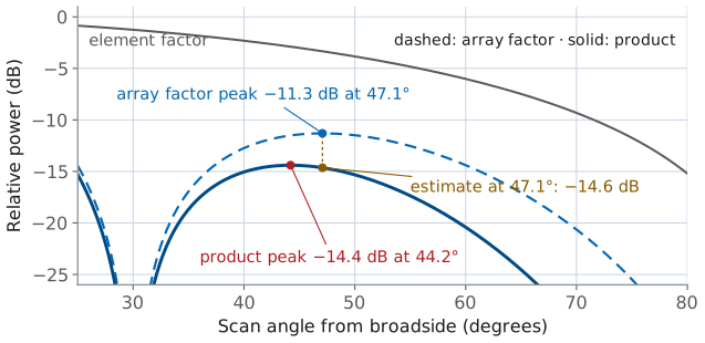
The first sidelobe of \(AF_4\) is −11.3 dB at 47.1°, where the element adds −3.3 dB.
The total is −14.4 dB at 44.2°; the main lobe narrows from 26.3° to 25.4°.
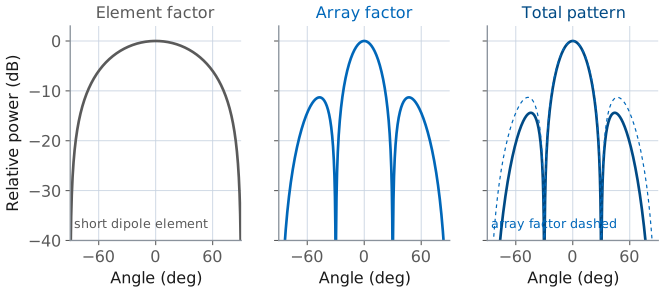
Worked example — four collinear short dipoles
Four short dipoles lie end to end along the array axis, spaced \(d = \lambda/2\), all fed in phase.
Lesson 7’s short dipole radiates as \(\sin\theta_{\text{polar}}\), which in scan angle is \(EF(\theta) = \cos\theta\): a broad lobe at broadside and a null along the array axis at \(\theta = \pm 90^\circ\).
The array factor is \(AF_4\) with \(\psi = \pi\sin\theta\). Its nulls fall at \(\sin\theta_m = m/2\), that is ±30° and ±90°, and its first sidelobe is −11.3 dB at \(\theta = \pm 47.1^\circ\).
At that angle the element factor is \(\cos(47.1^\circ) = 0.681\), or −3.3 dB. Adding the two levels in decibels estimates the total first sidelobe:
The product’s own peak sits slightly closer to broadside, at 44.2°, because the cosine is larger there, and its exact level is −14.4 dB. The estimate is within 0.2 dB.
The element factor did two things: it pushed the sidelobes down, more so the farther off broadside they sit, and it deepened the null at ±90° that the array factor already had. It changed the main lobe very little, because \(\cos\theta\) is flat near broadside: at the ±13.2° half-power edges of the array factor it is still 0.974, or −0.23 dB, so the half-power width narrows only from 26.3° to 25.4°.
The figure zooms in on that sidelobe. Adding the two levels at the array factor’s peak gives the amber point on the product curve; the product’s own peak, in red, sits 3° closer to broadside and 0.2 dB higher, because the array factor is flat at its own peak while the element factor keeps rising toward broadside.
The three-panel figure shows the general rule. A directive element reshapes the skirts of the pattern and suppresses whatever the array factor puts at wide angles, but the array factor sets the main lobe. It sets the beamwidth, and the element and the array share the wide-angle behavior.
Array Factor Builder
The widget below builds the array factor one control at a time. Start at the course array, \(N = 8\) and \(d/\lambda = 0.481\), and confirm the readouts against the closed-form table: half-power width 13.2°, first null 15.1°, first sidelobe −12.8 dB. Then sweep \(N\) and watch the beam narrow while the sidelobe level holds near −13 dB, since \(N\) sets the width and the shape of the excitation sets the sidelobes. Switch the element factor on to see pattern multiplication: the dashed \(\cos\theta\) envelope pulls the outer lobes down and leaves the main lobe alone. Then push \(d/\lambda\) toward 1.5 and watch a second full-height beam move in from the edge; Part 4 explains it.
Part 4: The Visible Region
Real angles reach only \(\psi_{\min}\) to \(\psi_{\max}\), the visible region.
Its width is \(2kd = 4\pi d/\lambda\); steering slides it without resizing it.
A second peak at \(\psi = \pm 2\pi\) radiates once the window reaches it.
\(AF_N(\psi)\) repeats every \(2\pi\) in \(\psi\), but \(\psi\) is not free: \(\psi = kd(\sin\theta - \sin\theta_0)\) ties it to a real angle. As \(\theta\) sweeps the visible half-space from −90° to +90°, \(\sin\theta\) covers −1 to +1, and \(\psi\) covers a window of total width \(2kd = 4\pi d/\lambda\) that slides as we steer. That window is the visible region, Lesson 6’s window \(-k \le k_z \le +k\) written in \(\psi\). Values of \(\psi\) outside it correspond to no real angle, so the array never radiates them.
The width of the window alone does not produce a second beam. At \(d = \lambda/2\) the window is exactly one period wide, and at broadside it runs from \(-\pi\) to \(+\pi\), between the repeats. A second copy of the main lobe appears only when an edge of the window reaches a repeat at \(\psi = \pm 2\pi\). At broadside the edges sit at \(\pm kd\), which reach \(\pm 2\pi\) when \(d = \lambda\). A copy that enters is a grating lobe, and because \(AF_N\) is exactly periodic it is as tall as the main lobe and radiates as much power as the intended beam.
Visible Region at Two Spacings
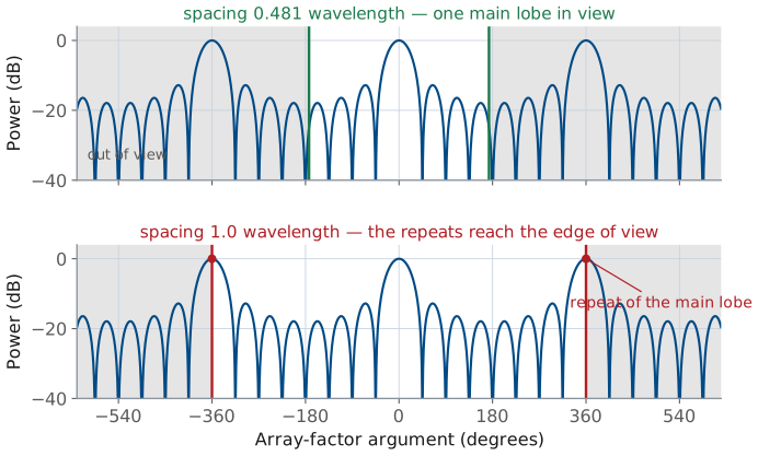
At \(d/\lambda = 0.481\) the window ends at ±173°, short of the repeats at ±360°.
At \(d = \lambda\) the edges reach ±360°, and full-height lobes appear at ±90°.
Visible Region Explorer
The top panel plots \(AF_N\) against \(\psi\) over several periods and shades the window that real angles reach; the bottom panel is the same pattern against scan angle. Start at the PHASER, \(d/\lambda = 0.481\), where the window spans ±173° and stops short of the repeats at ±360°. Widen the spacing and watch the window grow until its edges reach ±360° at \(d = \lambda\), and the repeats appear at ±90°. Then return to \(d/\lambda = 0.75\) and steer to 30°: the window slides without changing width, its left edge passes −360°, and a grating lobe appears at −56.4°.
Grating Lobes
At \(\psi = 2\pi m\) every element is back in phase with its neighbors.
Grating lobes appear where \(\psi\) is a nonzero multiple of \(2\pi\). At \(\psi = 2\pi\) the path difference between neighbors, less the applied progressive phase, is exactly one wavelength, so every term \(e^{\ jn\psi} = e^{\ j2\pi n} = 1\) and the elements add in phase exactly as they do at the main lobe. That is why a grating lobe is full height.
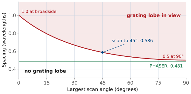
The grating lobe nearest real space is \(m = 1\) on the side away from the steer. For \(\theta_0 \ge 0\) it sits at \(\sin\theta_g = \sin\theta_0 - \lambda/d\), and it stays out of real space as long as \(\sin\theta_g < -1\):
A beam steered to negative \(\theta_0\) gives the mirror image, so the criterion carries \(\vert\sin\theta_0\vert\). At broadside it is \(d < \lambda\). Scanning to ±90° tightens it to \(d < \lambda/2\), which is where the familiar half-wavelength spacing comes from. The figure plots the limit against the largest scan angle a design needs: a ±45° requirement allows \(0.586\lambda\), and the PHASER’s \(0.481\lambda\) sits below the curve at every angle, so it can scan anywhere without a grating lobe. Lesson 23 treats grating lobes in full, alongside beam squint and phase quantization; we use the criterion as stated until then.
Note
Element spacing is a two-sided trade. Too large and a grating lobe appears. Too small and the array is short for its element count, so the beam is wide and the elements couple strongly to each other (mutual coupling, Lesson 21). Most designs land between \(0.4\lambda\) and \(0.5\lambda\).
Part 5: The Array as a Sampled Aperture
The array is a line source of length \(Nd\), sampled every \(d\), and \(Nd\) sets the beamwidth.
The excitation shape sets the sidelobes, −13 dB for uniform.
The spacing \(d\) decides whether a grating lobe reaches real space.
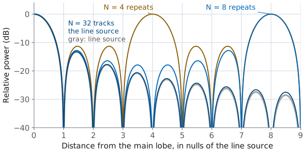
Near the main lobe and the first few sidelobes, \(\psi\) is a small fraction of a period when \(N\) is large, so the denominator \(N\sin(\psi/2)\) is close to \(N\psi/2\). The array factor then becomes \(\sin u/u\), with
for \(L = Nd\). That is the \(u\) of Lesson 6’s uniform line source, written in scan angle. A uniform line source of length \(L\) has a beamwidth \(\approx 0.886\ \lambda/L\) and a first sidelobe of −13.3 dB, and a uniform array of \(N\) elements spaced \(d\) has a beamwidth \(\approx 0.886\ \lambda/(Nd)\) and a first sidelobe near −13 dB. The array is that line source sampled every \(d\).
The figure shows where the approximation holds. Plotted against \(u\), in units of the line source’s null spacing, the 4-, 8-, and 32-element patterns all match the sinc near the main lobe. They part from it where \(\psi\) is no longer small: an \(N\)-element array repeats its main lobe at full height \(N\) nulls out, so the 4-element pattern returns at \(u/\pi = 4\) and the 8-element one at 8, while the 32-element pattern follows the sinc across the whole plot.
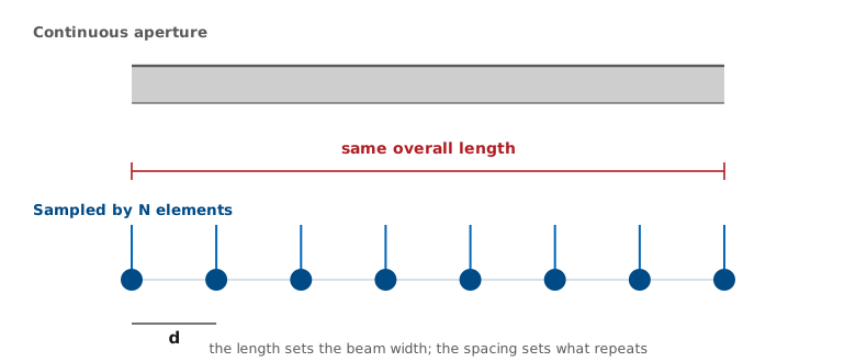
The sampled view assigns each parameter its job. Two arrays with the same \(Nd\) have nearly the same main lobe whether 8 elements or 32 fill that length. Uniform excitation gives about −13 dB in the array exactly as in the aperture, and Lesson 22 tapers it.
The spacing decides what repeats. The array samples the current only at multiples of \(d\), so its phases \(e^{\ jn\psi}\) cannot distinguish \(\psi\) from \(\psi + 2\pi\), and the pattern repeats with that period. Lesson 6 showed that the pattern is the Fourier transform of the current (“The Radiation Integral as a Fourier Transform”), and sampling a function makes its transform periodic. A continuous aperture has a contribution from every position, so no shift of \(\psi\) leaves all of them unchanged, and it has no grating lobes.
Worked Example: The Course Array
At 10.3 GHz, \(d = 14\) mm is \(0.481\lambda\), and \(Nd = 3.85\lambda\).
\(\psi\) spans ±173.2°, and \(d < \lambda/2\) rules out grating lobes.
Nulls fall at ±15.1°, ±31.3°, and ±51.2°; the half-power width is 13.2° and the first sidelobe −12.8 dB.
Worked example — the course 8-element array
The PHASER carries 8 patch elements spaced \(d = 14\ \text{mm}\). At 10.3 GHz, \(\lambda = 29.1\ \text{mm}\), so \(d/\lambda = 0.481\) and the array is \(Nd = 112\ \text{mm} = 3.85\lambda\) long.
Visible region. At broadside
so \(\psi\) runs over ±173.2°, a window just under one period wide whose edges stay well clear of the repeats at ±360°. The window holds no grating lobe. Because \(0.481 < 0.5\), the spacing criterion \(d < \lambda/(1 + \vert\sin\theta_0\vert)\) holds at every scan angle out to ±90°.
Nulls. \(\sin\theta_m = m\lambda/Nd = m/3.85\), giving ±15.1°, ±31.3°, and ±51.2°. The \(m = 4\) null would need \(\sin\theta = 1.04\), so it never reaches real space, and the array shows 6 sidelobes across the visible region.
Beam. The first-null and half-power beamwidths are
and the first sidelobe is −12.8 dB at ±21.9°. Lesson 20 derives the broadside directivity of a uniform array,
The Measured Sweep
The L20 Lab sweeps this beam past a fixed source. Expect a 13° beam, a first null past 15°, and sidelobes 11 to 13 dB down. The widget below is the one the L20 Lab uses: pick the 8-element aperture, read the half-power width, first-null width, and first sidelobe off the ideal curve, then switch the measurement effects on. The 2.8125° steer grid and the −23 dB noise floor fill in the nulls, and the first-null width moves from 30.1° to 28.1° because the grid no longer lands on the null.
Worked example — what the L20 Lab sweep will show
In the L20 Lab you will steer this array past a fixed source and record power against commanded angle. Expect a main lobe near 13° wide, a first null a little past 15°, and sidelobes 11 to 13 dB down. The measured beam reads 13.1°, and the nulls fill in: the sweep steps in 2.8125° increments and the receiver’s noise floor sits about 23 dB below the peak, so a mathematical zero measures as a finite dip.
Summary: The Array Factor and Its Closed Form
Idea |
Result |
|---|---|
Array factor |
\(AF = \sum a_n e^{jn\psi}\), one term per element |
Inter-element phase |
\(\psi = kd(\sin\theta - \sin\theta_0)\) |
Visible region |
±173° of \(\psi\) for the PHASER |
Uniform array |
\(\sin(N\psi/2)/(N\sin(\psi/2))\), peak 1 |
Nulls |
\(\psi = 2\pi m/N\) |
First sidelobe |
−13 dB (−12.8 dB at \(N = 8\)) |
Sidelobe count |
\(N - 2\) per period |
Summary: Multiplication and Spacing
Idea |
Result |
|---|---|
Pattern multiplication |
\(\vert F\vert = \vert EF\vert \times \vert AF\vert\), identical elements only |
Grating-lobe criterion |
\(d < \lambda/(1 + \vert\sin\theta_0\vert)\) |
Scan to 90° |
\(d < \lambda/2\) |
Beamwidth |
\(\approx 0.886\ \lambda/Nd\); 13.2° for the PHASER |
Practice
Looking Ahead
Lesson 17 covers the ADAR1000 hardware that sets each \(a_n\) in gain and phase.
Lesson 18 steers the beam to \(\theta_0\) with a phase ramp.
The L20, L22–L23, and L24 Labs measure this pattern, taper it, and place a null.
Today we assumed the feed: element \(n\) simply received weight \(a_n\). Lesson 17 opens the hardware that produces those weights, the ADAR1000 beamformer chips, the per-element gain and phase controls, and the receive chain that turns eight elements into two digitized channels. Lesson 18 then sets the weights to a progressive phase ramp and steers the beam, which supplies the \(\theta_0\) that has gone unused in \(\psi\) all lesson.
Every lab in this module measures some feature of today’s array factor. The L20 Lab measures the beamwidth, the nulls, and the sidelobe level of the uniform 8-element pattern. The L22–L23 Lab changes the weights and watches the sidelobes drop. The L24 Lab places a null where you want one. Before the next lesson, be able to write \(AF_N\) from memory and locate its nulls, because every one of those labs starts by predicting from it.