Lesson 21 separated the array factor from the pattern the array radiates and predicted where the two part company: the peak drops as \(\cos\theta_0\) when the beam steers, the two first sidelobes of a steered beam stop matching, and nothing comes out the back. Today we test those predictions on the bench. The L21 Lab packet starts from them: Part 1, the pre-lab you completed before class, works out the patterns at your HB100’s frequency and sizes the errors of the two methods. Today you measure the pattern twice with the beam held still, once by carrying the source around the array by hand and once by turning the kit in front of a fixed source. Part 3, on your own before Lesson 22, reconciles the numbers with the predictions and compares the two methods.

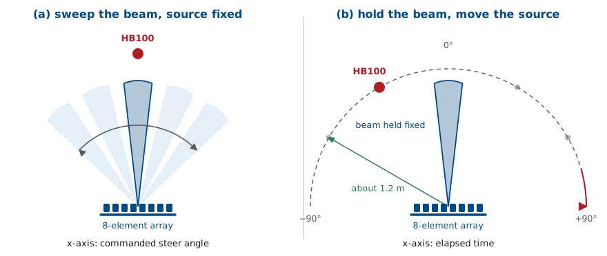
There are three ways to get a pattern out of an array, and they are not the same measurement.

The first is the one you have used since the L18 Lab: put a source somewhere, leave it there, and sweep the beam electronically past it, recording received power at each steer angle. The source sits at one physical angle, so the element pattern contributes the same constant to every point on the trace and drops out of its shape. The trace is the array factor, plotted against the angle the beamformer was commanded to.

The second is the one ADI’s workshop uses. Hold the beam fixed and carry the source around the array on an arc. Now the physical angle changes at every instant, so the element pattern multiplies the array factor exactly as Lesson 21 described, and the trace is the antenna pattern. The GUI plots it against elapsed time, though, so the angle axis is only as good as your walking, and the level is only as steady as your arm.

The third is what an antenna range does. Hold the beam fixed, leave the source on its tripod, and turn the kit in front of it. The trace is the antenna pattern again, but every reading carries a real angle, and the distance to the source never changes.

Part 1 of the packet works these out at your own kit’s frequency; the dBc values barely move with frequency, and the angles move by about 0.15° per 100 MHz, less than you can read off the stand’s scale. With the beam at 0° the element pattern lowers the ±21.4° sidelobes by only 0.3 dB, too little to see in a room. With the beam at 30° it lowers the peak by 0.6 dB and the outer sidelobe, near 59°, by 2.9 dB, while the inner one, near 8°, sits where the element is flat. The array factor alone would put both at −12.8 dBc. The ground plane removes the back hemisphere, so the reading with the source behind the board should sit at the floor.

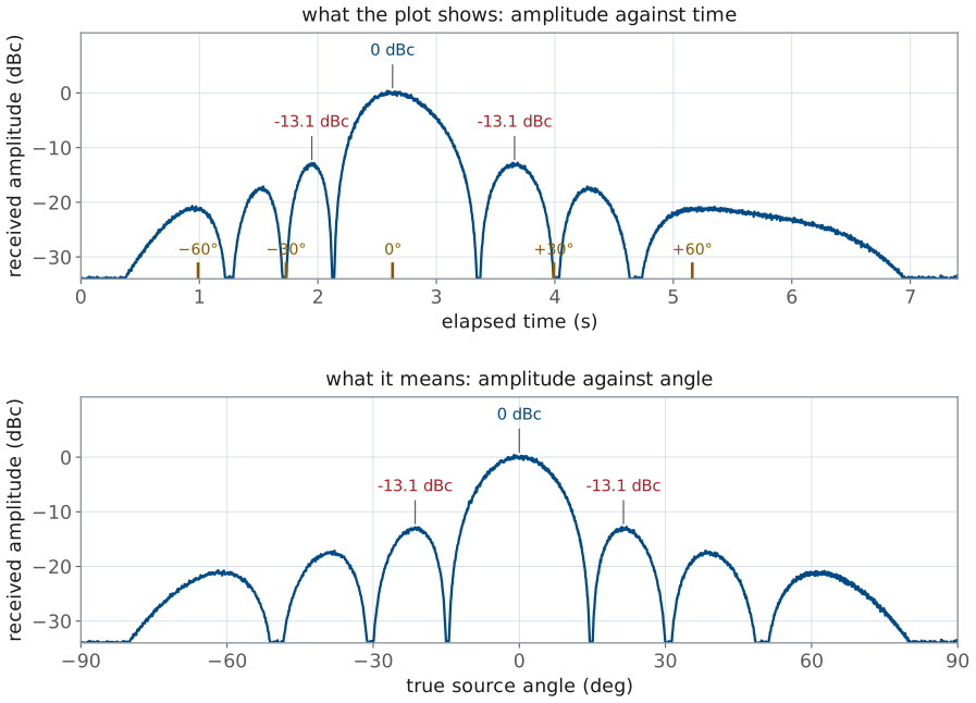
The level the GUI records at any instant is the pattern at the angle the source occupied at that instant, and it does not depend on how fast the source was moving. Walking slowly through a lobe draws it wider on the plot without changing its height, so the lobe levels survive an uneven walk and the angles do not. The level is not immune to your arm, though: received power goes as \(1/r^2\), so drifting 10 cm in or out at 1.2 m moves the reading by 0.7 to 0.8 dB, more than the scan loss you want to see. Three walks, compared in the packet, show how large that scatter is in practice.

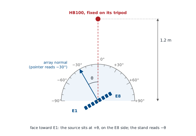
Turning the kit in front of a fixed source records the same pattern as walking the source around a fixed kit, because only the angle between the array normal and the source matters. What changes is everything else. The distance never changes, so the levels can be compared from one reading to the next; the HB100 stays aimed at the array without effort; and each reading is taken at an angle you can read off the stand’s scale, with a click every 5°.

Lesson 18 put \(+\theta\) on the E8 end of the array. Looking at the patches, E1 is at the right end of the row and E8 at the left. Turn the kit so that its face swings toward the E1 end, as seen from the source, and the source ends up on the E8 side of the normal, at \(+\theta\). The stand counts the other way: its scale is engraved on the fixed base and counts clockwise as seen from above, and turning the face toward E1 is a counterclockwise turn, so the pointer reads \(-\theta\). A source at +30° sits under a pointer reading −30. Part 2 starts by confirming that sign with a beam sweep, whose Angle readout, set to Peak, reads the source’s angle.

Two things set how good the rotation is. The kit must turn about the center of the array, between E4 and E5: an axis 20 mm off center moves the source’s apparent angle by up to 1° and its distance by up to 20 mm, about 0.14 dB. The stand puts the array’s center on its axis by design. And its scale, ticked every 5°, reads to a degree or two, which is fine for a lobe 15° wide.

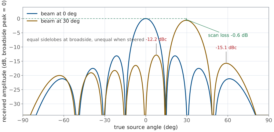
With the beam held at 30°, the main lobe appears when the source reaches about 30° instead of boresight. The peak reads lower than the broadside run, by 0.6 dB for the ideal element and about 0.9 dB for a real patch; the Module 3 dry run measured 0.7 dB with the source 1.2 m out. The rotation can resolve that difference because the distance never changes. A walk cannot, because the radius drift alone is as large as the effect.

The pattern is no longer symmetric. The first sidelobe on the inside of the beam, near +8°, sits about −12.2 dBc; the one on the outside, near +59°, sits about −15.1 dBc. The array factor alone would make them equal, and the element pattern lowers the outer one. A careful walk can show the direction of that 2.9 dB asymmetry; the rotation can put a number on it.

The packet’s Part 1 builds both budgets. The walk’s angle error comes from converting time to angle at a constant pace you did not have: a hand 30% fast or slow through the main lobe makes a 13.0° beam read anywhere from 10.0° to 18.6°. Its level error comes from the radius. The rotation removes both, and replaces them with the axis offset and the stand’s scale, which are small and can be measured. Neither method removes the room: a single reflection 18 dB below the direct path moves a reading by a decibel. The rotation’s advantage there is repeatability. The reflections sit in fixed places in the room, so a reading repeated at the same angle comes back to the same value, and a difference between two of them is more trustworthy than either reading alone.

You need the ADALM-PHASER kit on its rotating stand from the L17 Lab, connected to your laptop by the Ethernet cable as in Lesson 17; the HB100 with a fresh battery, on its tripod; and masking tape. Tape the stand’s base to the bench with its 0° mark toward the source, and seat the kit’s tripod in the platter’s grooves with the patches facing the pointer. A kit without a stand can use a printed protractor instead, centered under the middle of the array between E4 and E5 with 0° toward the source, but then mark it so that a turn toward E1 reads positive, and turn the tripod carefully about that center.

Set the HB100 1.2 m from the array face at the height of the patch row, facing the array. Lesson 21 put the far-field distance of this aperture at 0.67 m, but level comparisons of under a decibel need more distance: in the Module 3 dry run, scan loss read correctly at 1.2 m and only half of it at 1 m. Tape the walk’s arc on the floor at the same 1.2 m radius, with marks at −90°, 0°, and +90°.

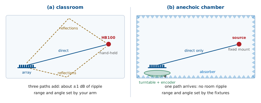
The rotation is a paper version of an antenna range, and comparing the two shows what the classroom still leaves in your data.

Angle. A range turns the antenna on a turntable with a shaft encoder, so every sample carries its angle to a fraction of a degree. Your sweep’s Angle readout gives each stop’s angle to about a degree, which the walk’s time axis cannot.

Distance. A range bolts the source at a fixed distance. So does the rotation; the walk does not.

Reflections. The direct path is not the only path from the HB100 to the array. Reflections off the floor, the ceiling, and the whiteboard arrive too and add to the direct signal in and out of phase, which is the ±1 dB of ripple in both of your methods. An anechoic chamber lines every surface with absorber so only the direct path survives.

Far field. You set 1.2 m against Lesson 21’s 0.67 m. A chamber satisfies the far-field condition only if it is long enough for the antenna and frequency; a large antenna in a short chamber has the same problem as a large antenna in a classroom.

You now have a measured −13 dBc in your packet, and so far it has been a fact about uniform illumination rather than a choice. Lesson 22 turns it into a design variable. Feeding the eight elements unequally, with more power in the middle and less at the edges, pushes the sidelobes down, and the Element Gains sliders you have been leaving at 100% are how you do it on this hardware.

A taper that lowers the first sidelobes by 10 dB widens the main lobe and lowers the peak gain, and Lesson 22 derives exactly how much of each. Before the next period, look back at your broadside rotation and decide how much beamwidth you would give up to put those first sidelobes at −25 dBc, then check your guess against the numbers.