Lesson 6 substituted \(V_0^- = \Gamma V_0^+\) into the wave solution on a lossless line, so one amplitude and the reflection coefficient describe the voltage everywhere. The current follows from Lesson 5: each wave’s current is its voltage divided by \(Z_0\), with a minus sign on the reflected wave because it travels in the \(-z\) direction. The load sits at \(z = 0\) and the source end of the line at \(z = -\ell\). Today we evaluate both at the source end.

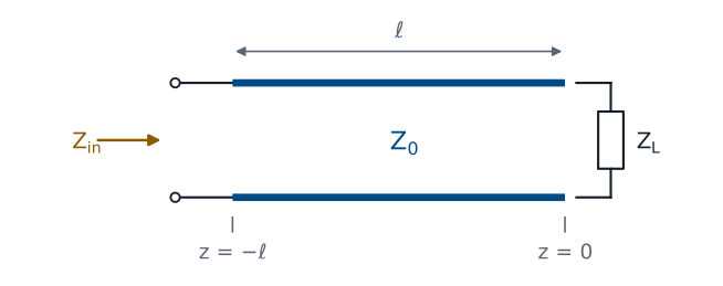
The source does not connect to the load; it connects to the line. What the source sees at its terminals is the ratio of the total voltage to the total current at \(z = -\ell\), which we call the input impedance \(Z_\text{in}\). If we replaced the line and the load with a single impedance equal to \(Z_\text{in}\), the source could not tell the difference: it would deliver the same current and the same power. That equivalence is what makes \(Z_\text{in}\) useful. It reduces any line and load to one impedance in the source’s circuit.

We substitute \(z = -\ell\) into the voltage and current. Each \(e^{-j\beta z}\) becomes \(e^{+j\beta\ell}\), and each \(e^{+j\beta z}\) becomes \(e^{-j\beta\ell}\). The amplitude \(V_0^+\) appears in both the numerator and the denominator, so it cancels, and \(Z_0\) moves from the denominator’s denominator to the front. The input impedance does not depend on how hard the source drives the line, only on \(Z_0\), \(\Gamma\), and the electrical length \(\beta\ell\). This form is already useful, and Lesson 10 builds the Smith chart on it.

To write the result in terms of the load, we substitute \(\Gamma = \frac{Z_L - Z_0}{Z_L + Z_0}\) and multiply the numerator and denominator by \(Z_L + Z_0\), which clears the fraction inside a fraction. Next we collect the terms that multiply \(Z_L\) and the terms that multiply \(Z_0\). In the numerator, \(Z_L\) multiplies \(e^{+j\beta\ell} + e^{-j\beta\ell} = 2\cos\beta\ell\) and \(Z_0\) multiplies \(e^{+j\beta\ell} - e^{-j\beta\ell} = 2j\sin\beta\ell\), by Euler’s identity; the denominator works the same way with the roles of \(Z_L\) and \(Z_0\) exchanged. Finally we divide every term by \(2\cos\beta\ell\). The result is the transmission line equation for a lossless line.

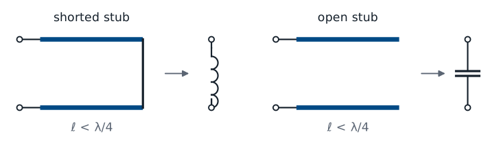
For a short circuit we set \(Z_L = 0\) directly. For an open circuit we cannot substitute infinity, so we first divide the numerator and denominator by \(Z_L\) and then let \(Z_L \to \infty\), which removes every term with \(Z_0/Z_L\). Both results are purely imaginary: a line terminated in a short or an open dissipates nothing, so it can only store energy, and its input impedance is a pure reactance. Which reactance depends on the length. A shorted line shorter than \(\lambda/4\) has positive reactance, like an inductor; an open line shorter than \(\lambda/4\) has negative reactance, like a capacitor.

A short length of line with a short or an open at its end is called a stub, and at microwave frequencies stubs replace inductors and capacitors, which are hard to build with accurate values above a few gigahertz. A shorted stub \(\lambda/8\) long has \(\tan\beta\ell = 1\), so \(Z_\text{in} = j50\ \Omega\) on a \(50\ \Omega\) line. In RG-58 at 1 GHz, \(\lambda = v_p/f = 20\) cm, so the stub is 2.5 cm long, and it presents the same reactance as an inductor with \(L = \frac{50}{2\pi \times 10^9} = 7.96\) nH. The stub’s reactance changes with frequency differently than an inductor’s, so the equivalence holds at one frequency. Lesson 9 uses stubs to build matching networks.

A matched line has no reflected wave, so the ratio of voltage to current is \(Z_0\) everywhere, and the input impedance is \(Z_0\) at any length. A half-wave line, \(\ell = \lambda/2\), has \(\beta\ell = \pi\) and \(\tan\beta\ell = 0\), so the input impedance equals the load impedance, whatever the load. The same holds for any whole number of half wavelengths. A half-wave line is transparent: it moves the load to a new location without changing what the source sees, at the frequency where it is exactly \(\lambda/2\) long.

At \(\ell = \lambda/4\), \(\beta\ell = \pi/2\) and \(\tan\beta\ell\) is infinite, so we divide the numerator and denominator by \(\tan\beta\ell\) before taking the limit. The terms divided by \(\tan\beta\ell\) vanish, and what remains is \(Z_0^2/Z_L\). A quarter-wave line inverts the load impedance about \(Z_0\): a short becomes an open, an open becomes a short, and a \(25\ \Omega\) load on a \(50\ \Omega\) line looks like \(50^2/25 = 100\ \Omega\).

The inversion gives a simple way to match a resistive load. We insert a quarter-wave section of a different line, with characteristic impedance \(Z_1\), between the main line and the load. Seen through the section, the load becomes \(Z_1^2/R_L\), and setting that equal to \(Z_0\) gives \(Z_1 = \sqrt{Z_0 R_L}\), the geometric mean of the two impedances. To match a \(100\ \Omega\) load to a \(50\ \Omega\) line, the section needs \(Z_1 = \sqrt{50 \times 100} = 70.7\ \Omega\). The match is exact only at the frequency where the section is \(\lambda/4\) long, and it works only for a real load; Lessons 8 and 9 handle complex loads.

The time-average power carried past any point is one half the real part of the voltage phasor times the conjugate of the current phasor, the same rule as in circuit analysis. We substitute both phasors; conjugating the current flips the sign of every exponent and conjugates \(\Gamma\). Multiplying out gives four terms. Two of them are \(1\) and \(-\vert\Gamma\vert^2\), both real. The other two are a number and minus its own conjugate, which is purely imaginary, so the real part removes them. What remains does not depend on \(z\).

The first factor is the power the incident wave carries by itself, and the reflected wave carries \(\vert\Gamma\vert^2\) of it back toward the source. The net power is the same at every point, which is what conservation of energy requires on a lossless line: none is lost along the way, so whatever passes the source end must arrive at the load. This is the derivation behind the rule Lesson 6 used, that a load absorbs \(1 - \vert\Gamma\vert^2\) of the incident power.

The quarter-wave transformer matches a real load, but most loads are complex. The widget showed that along any mismatched line there are points where the input resistance equals \(Z_0\) exactly, and only a reactance is left over. Lesson 8 finds those points from the magnitude and phase of \(\Gamma\), then cancels the leftover reactance with a capacitor or inductor in series. Lesson 9 does the same with admittances and a component in parallel, then replaces the component with one of today’s stubs.

Before Lesson 8, read sections 3.21 through 3.23 of Ellingson, Electromagnetics, Vol. 1.