Lesson 4 turned the telegrapher’s equations into phasor form, uncoupled them into a wave equation, and solved it. The voltage is an incident wave with amplitude \(V_0^+\) traveling toward the load and a reflected wave with amplitude \(V_0^-\) traveling toward the source. The current has the same form with its own constants, \(I_0^+\) and \(I_0^-\). Those four constants are not independent, because the voltage and current must still satisfy the first-order phasor equation shown here. That equation is where we start.

We differentiate the voltage solution with respect to \(z\). Each exponential \(e^{\mp\gamma z}\) brings down a factor of \(\mp\gamma\), and the minus sign on the left side flips both signs. The first-order phasor equation says this same quantity equals \(\left(R' + j\omega L'\right)\widetilde{I}(z)\), so we set the two equal and divide by the series impedance. The result gives the current everywhere on the line in terms of the voltage constants alone. The two waves appear with opposite signs: the reflected wave’s current flows in the \(-z\) direction, the direction it travels.

The factor \(\gamma/(R' + j\omega L')\) has units of inverse ohms, so we define its reciprocal as the characteristic impedance \(Z_0\). Writing \(\gamma\) as its square root, the series impedance appears once in the numerator and once under the root in the denominator, and dividing leaves the square root of the series impedance over the shunt admittance. Replacing the factor with \(1/Z_0\) in the current solution and comparing with \(\widetilde{I}(z) = I_0^+ e^{-\gamma z} + I_0^- e^{+\gamma z}\) term by term gives the two current constants. In the incident wave, voltage and current are in the ratio \(Z_0\); in the reflected wave, the ratio is \(-Z_0\).

The characteristic impedance is easy to misread as the impedance of the line, so it is worth stating what it is. It is the ratio of voltage to current in a single traveling wave. It depends only on \(R'\), \(L'\), \(G'\), and \(C'\), which depend only on the cross section and the materials, so every length of RG-58 has the same \(Z_0\). It does not dissipate power the way a resistor does; on a lossless line, the power carried by the wave simply moves down the line. If the line were infinitely long, no wave would ever come back, so a source connected to it would see only the incident wave and measure an impedance of exactly \(Z_0\). Once a reflected wave is present, the ratio of total voltage to total current changes along the line, and Lesson 7 computes it.

Lesson 4 showed that a crest of the incident wave moves in the \(+z\) direction. To find how fast, we set its phase, \(\omega t - \beta z\), equal to a constant, which describes the crest’s position as a function of time. Differentiating both sides with respect to \(t\) gives \(\omega - \beta\ dz/dt = 0\), and solving for \(dz/dt\) gives the speed of the crest. That speed is the phase velocity \(v_p\), the speed at which any point of constant phase moves along the line.

At a fixed instant, the cosine \(\cos(\omega t - \beta z)\) repeats each time \(\beta z\) advances by \(2\pi\). The distance over which that happens is the wavelength, so \(\beta\lambda = 2\pi\). This is the physical meaning of the phase constant: \(\beta\) is the phase change per meter, and there are \(2\pi\) radians in each wavelength. Substituting \(\beta = \omega/v_p\) and \(\omega = 2\pi f\) recovers \(\lambda = v_p/f\), the relation Lesson 3 used to decide when a line is electrically long.

Lesson 4 found \(\alpha = 0\) and \(\beta = \omega\sqrt{L'C'}\) for a lossless line. Dividing \(\omega\) by \(\beta\) cancels the frequency, so the phase velocity on a lossless line is the same at every frequency. In the characteristic impedance the factors of \(j\omega\) cancel too, so \(Z_0\) is a real number, independent of frequency. For RG-58, with \(L' = 259\) nH/m and \(C' = 96.8\) pF/m,

These are the velocity Lesson 3 quoted and the impedance Lesson 6 derives from the cable’s dimensions.

Real cables have small losses, and we want \(\alpha\) without carrying the full square root. We factor \(j\omega L'\) out of the series impedance and \(j\omega C'\) out of the shunt admittance, which pulls out the lossless \(\gamma\) and leaves two square roots of the form \(\sqrt{1 + x}\), where \(x\) is small. For small \(x\), \(\sqrt{1 + x} \approx 1 + x/2\), the first two terms of its Taylor series. Multiplying out the two factors produces a term with the product of two small quantities, which we drop. Multiplying \(j\omega\sqrt{L'C'}\) through the remaining terms, the \(j\omega\) cancels in each correction, and they come out real.

The real part of \(\gamma\) is the attenuation constant. Recognizing \(\sqrt{L'/C'}\) as the lossless \(Z_0\), the conductor term is \(R'/2Z_0\) and the dielectric term is \(G' Z_0/2\). The imaginary part is unchanged from the lossless line, so to first order the losses change how fast the wave decays but not its speed or wavelength. The voltage amplitude falls by \(e^{-\alpha\ell}\) over a length \(\ell\). Expressing the ratio in decibels, \(20\log_{10} e^{\alpha\ell} = 20\alpha\ell\log_{10} e\), and \(20\log_{10} e = 8.686\), so one neper is \(8.686\) dB.

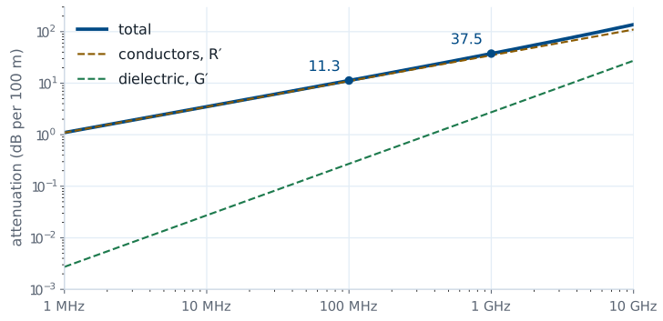
The figure plots the two terms of \(\alpha\) for RG-58 from 1 MHz to 10 GHz. The conductor term rises as the square root of frequency, because \(R'\) does: at higher frequency the current crowds into a thinner layer at the surface of each conductor, and less copper carries it. The dielectric term rises in direct proportion to frequency, because \(G' = \omega C' \tan\delta\), where \(\tan\delta = 2 \times 10^{-4}\) is the loss tangent of polyethylene. For this cable, the conductors dominate across the whole range. The total goes from \(11.3\) dB per 100 m at 100 MHz to \(37.5\) dB per 100 m at 1 GHz.

The lossless model is a good approximation whenever \(\alpha\ell\) is small. A 2 m cable on the bench at 100 MHz loses \(0.113 \times 2 = 0.23\) dB, about 5% of the power, which is why the labs in this module treat their cables as lossless. A 30 m run from a radio to a rooftop antenna at 1 GHz is different: even the ideal model gives \(0.375 \times 30 = 11\) dB, so less than a tenth of the transmitter’s power reaches the antenna. That is why long runs at high frequency use larger, lower-loss cable, and why a link budget always includes the cable.

We now have a complete description of waves on an unterminated line: the current in each wave, its speed, its wavelength, and its loss. Every one of those depends on the line alone. Lesson 6 adds the load. At the load, the ratio of total voltage to total current must equal \(Z_L\), and unless \(Z_L = Z_0\), a single incident wave cannot satisfy that condition. A reflected wave appears, and its size relative to the incident wave is the reflection coefficient.

Before Lesson 6, read sections 3.10 and 3.12 through 3.14 of Ellingson, Electromagnetics, Vol. 1.