Circuit theory describes a network with voltages and currents at a handful of nodes. Electromagnetics describes the fields everywhere in space: the electric field between two conductors, the magnetic field around a current, and the way each one changes when the other does. When a circuit is small compared to the wavelength of its signals, the fields settle everywhere in the circuit at essentially the same instant, and the voltages and currents at the nodes are all we need. When it is not, the fields take time to travel, and we need the full theory. This course builds that theory and shows exactly where the circuit model fails.

Almost every system an Air Force engineer touches moves information with electromagnetic waves. A radar transmits a wave and measures what reflects; GPS receivers time waves from satellites; data links, satellite communications, and cellular and Wi-Fi networks all send waves through the air. Inside each of those systems, the signals move through hardware that electromagnetics governs: the coaxial cable from a radio to its antenna, the microstrip traces on a circuit board, the twisted pairs in a network cable. Electromagnetic testing also finds cracks and corrosion in aircraft structures without taking them apart. In each case, the questions are the same ones this course answers: how a signal travels, how much of it reflects, and how much arrives.

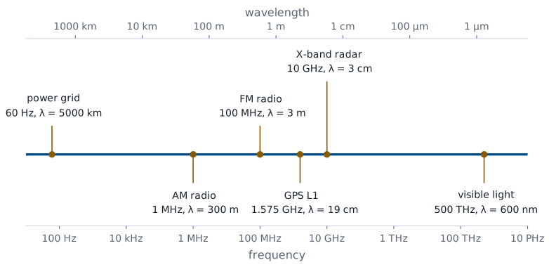
Every one of these systems uses the same physics at a different frequency. The wavelength in free space is the speed of light divided by the frequency, so the spectrum runs from the 5000 km wavelength of the 60 Hz power grid to the 600 nm wavelength of visible light. The wavelength sets the scale on which electromagnetic effects appear. A GPS signal at 1.575 GHz has a 19 cm wavelength, the size of a handheld receiver; an X-band radar at 10 GHz has a 3 cm wavelength, which is why its antenna elements are a few centimeters across. Lesson 3 uses the same ratio to decide when a wire stops behaving like a wire.

Four equations describe every electromagnetic effect in this course. Gauss’s law says electric charge is the source of electric flux. Gauss’s law for magnetism says magnetic flux has no source: magnetic field lines always close. Faraday’s law says a changing magnetic field produces a circulating electric field, which is how a transformer and a generator work. Ampere’s law says a current, or a changing electric field, produces a circulating magnetic field. The last two together are what let a wave exist: each changing field creates the other. Lesson 2 defines the four fields in these equations, Modules 2 and 3 build each law from experiment, and Module 4 puts them together.

Circuit laws are special cases of Maxwell’s equations. Faraday’s law in integral form says the line integral of the electric field around a closed path equals the negative rate of change of the magnetic flux \(\Phi\) through the path. Around a circuit loop, the line integral of \(\mathbf{E}\) across each element is the voltage across that element, so the left side is the sum of the voltages around the loop. When the loop is small and the magnetic flux through it changes slowly, the right side is negligible, and the result is Kirchhoff’s voltage law. At high frequency, or in a large loop, the flux term no longer vanishes, and neither does the sum of the voltages.

Charge is conserved, so the net current flowing out through any closed surface equals the rate at which the charge inside it decreases. Wrapping the surface around a circuit node, the surface integral of the current density is the sum of the currents leaving the node. When no charge builds up at the node, the right side is zero, and the result is Kirchhoff’s current law. On a transmission line, charge does build up along the conductors as the wave passes, and Lesson 3 shows how the line’s capacitance accounts for it.

The course starts where circuit theory first fails: the transmission line, the place a cadet is most likely to meet electromagnetics on a bench. Module 1 treats it with voltages and currents, and it ends with a lab on a network analyzer. Modules 2 and 3 then build the field theory underneath, starting with the vector calculus it needs: the electric field of charges at rest, and the magnetic field of steady currents. Module 4 lets the fields change in time, completes Maxwell’s equations, and finds the uniform plane wave, the wave that carries a radar pulse or a GPS signal through the air. Each module has a lab.

Every learning objective has an assessment, scored on a binary scale: a 1 means you have mastered the objective, and a 0 comes with feedback. If you made a real attempt on time, you may revise your work until you earn the 1. The two graded reviews and the final exam are individual and graded on a specification scale of 0, 0.5, or 1 per problem. Engagement rewards the practice problem sets, extra instruction, and an optional research paper. The syllabus has the details, the policies, and the full schedule.

Each lesson page is both the slides and the notes. In present mode it shows the key points and equations we work through in class; in read mode, the default, it adds the full explanation and every step of each derivation. The course text is Ellingson, Electromagnetics, Vol. 1, which is free online, and each lesson ends with the sections to read before the next one. Each lesson also has a practice set, with a blank copy to work and a solutions copy to check against. The materials page collects the text, the equation sheet, the Smith charts, and every handout in one place.

Lesson 2 sets up the tools every later lesson uses. It defines scalar and vector fields, describes a wave mathematically, and develops phasors, which turn every sinusoidal signal into a single complex number. It then defines the electric and magnetic fields and flux densities in Maxwell’s equations, and the material properties that connect them. With those in hand, Lesson 3 takes up the transmission line.

Before Lesson 2, read Chapter 2 of Ellingson, Electromagnetics, Vol. 1.