Last lesson every load was a single impedance on port 1, so the only quantity that mattered was \(S_{11}\). The open, the short, and the capacitor dissipated nothing and reflected everything; the \(1\ \text{k}\Omega\) resistor reflected most of the wave; the series resistor and capacitor reflected less as the frequency rose; the matched load reflected almost none of it. A filter has two ports, so today the wave that gets through, \(S_{21}\), matters as much as the wave that comes back.

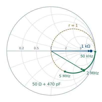
Each point on the chart is a value of \(\Gamma\), and the ray from the center to it has length \(\vert\Gamma\vert\) and angle equal to the phase of \(\Gamma\). The \(1\ \text{k}\Omega\) resistor has \(z = 20\), a real impedance, so it sits on the real axis at \(\Gamma = 0.905\angle 0^\circ\), and it stays there at every frequency because a resistor’s impedance does not change with frequency. The complex load, the \(50\ \Omega\) resistor in series with the 470 pF capacitor, has \(r = 1\) at every frequency, so it moves along the \(r = 1\) circle. At 50 kHz its reactance is \(-j6773\ \Omega\) and it sits near the open. As the frequency rises the reactance shrinks, and the point moves down the circle toward the center: \(0.861\angle -30.6^\circ\) at 2 MHz and \(0.561\angle -55.9^\circ\) at 5 MHz. A series inductor with the opposite reactance would carry it the rest of the way to the center, the series match of Lesson 12.

The DUT sits between the analyzer’s two ports. Port 1 launches the incident wave, and the analyzer measures two ratios at each frequency: the reflected wave over the incident wave, \(S_{11}\), and the transmitted wave over the incident wave, \(S_{21}\). Port 2 is a matched receiver, so it absorbs the transmitted wave, and nothing bounces back into the DUT. \(S_{21}\) is the transmission coefficient for the whole device, the two-port counterpart of the \(T = 1 + \Gamma\) of Lesson 6.

A filter built from inductors and capacitors stores energy but dissipates almost none, so every bit of power the incident wave carries in must leave as either the reflected wave or the transmitted wave. Each wave travels on a line of impedance \(Z_0\), so its power is its amplitude squared over \(2Z_0\), the result of Lesson 7. We write the balance, cancel the common factor \(\vert a\vert^2/2Z_0\), and get the result. A filter does not absorb the frequencies it rejects; it reflects them. Where \(\vert S_{21}\vert\) is near \(0\) dB, \(\vert S_{11}\vert\) is low, and where \(\vert S_{21}\vert\) falls, \(\vert S_{11}\vert\) rises toward \(0\) dB.

The passband is where \(\vert S_{21}\vert\) sits near \(0\) dB, and the stopband is where it falls far below. Sweep wide enough to see both, then read the type off the blue \(\vert S_{21}\vert\) trace. The yellow \(\vert S_{11}\vert\) trace should mirror it, low where the filter passes and near \(0\) dB where it rejects. A real filter has a little loss, so \(\vert S_{21}\vert\) in the passband reads a fraction of a dB below zero.

The cutoff frequency is the edge of the passband, defined as the frequency where the transmitted power falls to half its passband value. Power goes as the square of the wave amplitude, so half the power means an amplitude ratio of \(1/\sqrt{2}\). Converting with \(20\log_{10}\) gives \(-3\) dB, which is why the cutoff is called the \(-3\) dB point. Set a marker on the \(\vert S_{21}\vert\) trace and move it until it reads \(3\) dB below the passband level. A band-pass or band-stop filter has two such points. For a lossless filter, the power balance puts \(\vert S_{11}\vert\) at \(-3\) dB at the same frequency.

The Smith chart marker reads the impedance the DUT presents at port 1. The sign of the reactance tells you which kind of element the DUT looks like at that frequency: negative in the lower half of the chart, capacitive; positive in the upper half, inductive. To get the equivalent element value, we set the measured \(X\) equal to the reactance of a capacitor or an inductor and solve. A capacitor has \(X = -1/(\omega C)\), so \(C = -1/(\omega X)\). An inductor has \(X = \omega L\), so \(L = X/\omega\). The value describes the DUT at that one frequency only; as the marker moves, the equivalent value changes, because a filter is a network of several elements, not one.

Suppose the marker reads \(42 - j30\ \Omega\) at 10 MHz. The reactance is negative, so the DUT looks capacitive there, and \(C = -1/(\omega X) = 1/(2\pi \times 10^7 \times 30) = 531\) pF. If at the same frequency it read \(55 + j40\ \Omega\) instead, the DUT would look inductive, with \(L = 40/(2\pi \times 10^7) = 637\) nH. In the lab, record the frequency range over which the trace stays in each half of the chart, and one equivalent value in each range.

This lab closes Module 1. Everything so far has lived on a transmission line, where voltage and current along one coordinate tell the whole story. Module 2 steps off the line into three-dimensional space, where the electric and magnetic fields are vectors that vary in every direction. Lesson 17 reviews the vector algebra and the three coordinate systems the rest of the course uses.

Before Lesson 17, read Chapter 4 of Ellingson.