L15 Lab — mPSK#
mPSK
Build a carrier-recovery loop, turn up the noise until each constellation breaks, find the Costas Loop’s limits, and send QPSK through a PlutoSDR.
L15 Lab · Module 6: Waveform Applications & RF Reverse Engineering · Dr. Neil Rogers
Learning Objectives
- I can implement an mPSK modulator and demodulator (BPSK, QPSK, 8PSK) and recover carrier and symbol timing.
From Lesson to Bench
Pre-Lab: run the link and work out the settings the bench needs.
Bench: build a Costas Loop, find the noise, offset, and phase limits, then use a PlutoSDR.
Writeup: explain the noise order, the pull-in limits, and differential coding.
Lesson 15 built an mPSK text link with timing and carrier recovery, following the GNU Radio wiki’s Guided Tutorial PSK Demodulation. Today you first build an 8PSK carrier-recovery loop yourself, then raise the noise until each constellation stops delivering text, find the Costas Loop’s pull-in range, map its phase ambiguity, and then run QPSK on a PlutoSDR. The lab takes most of the lesson’s second period. The lab packet has three parts, and you turn it in once, complete, before Lesson 16. Part 1, the Pre-Lab, is on your own before the period: run L15-psk-link.grc once and work out the block settings Part 2 needs. Part 2 is your own measurements in class. Part 3, the Writeup, explains them.
Questions 1 to 6 run on your laptop and transmit nothing. Question 7 transmits, into a cable only, as the PlutoSDR frame below describes.
Part 1: Before the Period
L15-psk-link.grcruns and shows the received line.Work out the 8PSK point angles and the Costas frequency scale for your build.
Do the Pre-Lab before you arrive. Question 1 checks that the link flowgraph opens and runs on your laptop, and has you type a 50 Hz frequency offset to see the ring of the lesson’s opening figure: if GRC reports an error, the L5 lesson page lists the install checks, and EI before the lab is the place to fix it.
Question 2 asks for the settings the bench needs: the angles of the eight 8PSK points for your Chunks to Symbols table, the constant that turns the Costas Loop’s frequency output into hertz, and how far a 20 Hz offset turns the constellation each symbol.
Part 2: Build a Carrier-Recovery Loop
Start GRC and choose File, New, QT GUI. Do not open the lesson’s flowgraphs; build this one yourself.
Set
samp_rateto 4000, one sample per symbol. Add an Import block withimport math, cmath, a Variableptsholding the eight 8PSK points from your Question 2(a) table, in order, as a list of complex numbers (cmath.exp(1j*math.radians(a))is the point at angleadegrees), and a QT GUI Rangefoff: label Frequency offset (Hz), default 20, start \(-200\), stop 200, step 5.Add a Random Source: type byte, minimum 0, maximum 8, number of samples 10000, repeat Yes. Then Chunks to Symbols: input byte, output complex, symbol table
pts. Then a Throttle: type complex, sample ratesamp_rate.Add a Signal Source: type complex, sample rate
samp_rate, waveform Cosine, frequencyfoff, amplitude 1. Add a Multiply with 2 complex inputs and connect the Throttle and the Signal Source to it. This is the frequency offset.Add a Noise Source: type complex, Gaussian, amplitude 0.2, and an Add with 2 complex inputs. Connect the Multiply and the Noise Source to the Add.
Add a Costas Loop: loop bandwidth 0.02, order 8. Connect the Add’s output to it.
Add a QT GUI Constellation Sink with 2 inputs: the Add’s output to input 0 and the Costas Loop’s first output to input 1. Add a Multiply Const: type float, constant your Question 2(b) constant, on the Costas Loop’s frequency output, and a QT GUI Number Sink on that, with minimum \(-200\) and maximum 200. Every arrow must be black.
Run it. Screenshot the canvas for Question 3(a) and the window for Question 3(b). Record the frequency reading at 20 Hz, then type \(-60\) into the offset box and record it again.
Stop the flowgraph, set the Costas Loop’s order to 2, run it again, and describe the output for Question 3(c).
Part 2: Noise
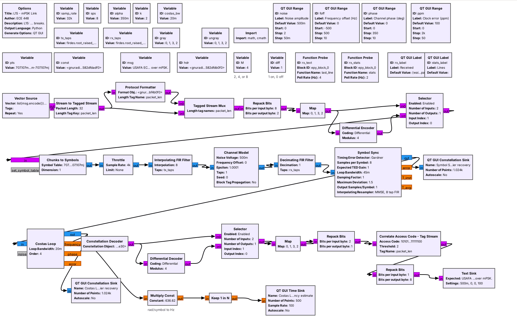
Open and run
L15-psk-link.grcwith every slider at its default: noise amplitude 0.5, no frequency offset, channel phase 0, anddiff= 1, differential coding on. The Lines label counts the lines received, and the correct ones, since a slider last moved.Start at the default noise amplitude of 0.5. Wait about 20 s and watch the Costas Loop’s output and the Lines label. Raise the noise by 0.1 at a time, typing each value into the noise amplitude box and pressing Enter, until only about half the lines received are correct, and record that noise amplitude for Question 4(a).
Stop the flowgraph. Double-click the variable
M, set it to 2, and run it again. Repeat step 2.Stop it, set
Mto 8, and run it again. Repeat step 2. Screenshot the window at that noise amplitude for Question 4(c).
Part 2: Carrier Recovery
Stop the flowgraph, set
Mto 4 anddiffto 1, and run it again, with the noise amplitude at its default of 0.5.With the frequency offset at 0 and lines arriving, type 250 into the frequency offset box in one jump. Watch the frequency estimate for up to 20 s, and record whether the loop locks, about how long it takes, and the frequency it settles at, for Question 5(a).
Type 0, wait until lines arrive again, and repeat step 2 for 350 and then 400 Hz. At any offset where the loop does not lock, record where its estimate settles and count the clusters in the Costas Loop’s output.
Stop the flowgraph, set
Mto 8, and run it again. Type 100 into the frequency offset box and record the same three things for Question 5(b). For 150, 200, and 250 Hz, stop the flowgraph and run it again before each one, so the loop starts locked at 0 Hz; returning to 0 by typing can leave the 8PSK loop stuck.
Part 2: Phase Ambiguity
Stop the flowgraph, set
Mto 4 anddiffto 0, and run it again, so the loop locks with no frequency offset and the channel phase at 0. Do not move the frequency offset or the noise in this part. Lines should keep arriving.Record whether lines arrive at phase 0. Then type 20 into the channel phase box. Record whether the Lines count keeps rising after about 5 s. Then type 0, wait until the Lines count rises again, and type the next phase.
Repeat for every phase from 20 to 340 in steps of 20, returning to 0 between them, for Question 6(a).
Stop the flowgraph, set
Mto 8, keepdiffat 0, and run it again. Repeat steps 2 and 3, but stop the flowgraph and run it again before each phase instead of typing 0: the 8PSK loop can slip to another rotation, and typing 0 does not bring it back.Stop the flowgraph, set
diffto 1, run it again, and repeat three of the phases that failed, for Question 6(b).Stop the flowgraph, set
Mto 4 anddiffto 0, and run it again. Step the phase from 0 to 100 by 20 at a time without returning to 0, and record what happens for Question 6(b). Setdiffback to 1 when you finish.
If No Text Arrives
If the Received label stays at “(waiting for a packet)”
Close the flowgraph and run it again with the sliders at their defaults, where every line should arrive within a second. With diff = 0, text arrives only when the loop has locked in the right rotation, and any frequency offset or phase jump you applied during the run can leave it locked in another one; run the flowgraph again with the sliders at their defaults. After a phase jump, judge by whether the Lines count keeps rising, not by the Received label: one packet already in the receiver can still arrive after a jump that fails. If the Costas Loop’s output keeps turning, the frequency offset is beyond its pull-in range: type 0 and wait. If you changed M, check that it is 2, 4, or 8 and that you ran the flowgraph again. In your own carrier-recovery flowgraph, check that the Costas Loop’s order is 8 and that the Signal Source’s sample rate is samp_rate.
Part 2: QPSK on a PlutoSDR
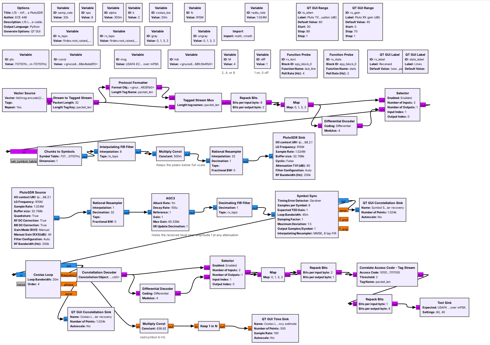
You cable one Pluto’s TX port to its RX port through a 30 dB attenuator, at 915 MHz.
Connect the cable before the flowgraph runs, and never connect an antenna.
L15-psk-pluto.grc is the Lesson 15 link with the Channel Model replaced by a PlutoSDR. The transmit half raises the 32 kHz stream to 1.024 MS/s and sends it from the Pluto’s TX port at 915 MHz; the receive half takes it from the RX port, lowers it to 32 kHz, and runs the same matched filter, Symbol Sync, Costas Loop, and decoder. The received level depends on the cable, the attenuator, and the gain, and it is far weaker than in the simulated link, so an AGC after the resampler holds it near amplitude 1. The Pluto’s transmitter and receiver share one reference oscillator, so the frequency offset is close to zero, but the carrier’s phase at the receiver changes every time the flowgraph starts. We have run this flowgraph only in simulation, with a model of the cable in place of the radio, so your bench is its first run on hardware.
In class we transmit only into a cable, into a shielded enclosure, or at very low power in an ISM band, and only when the lesson says to. This question transmits only into the cable between the Pluto’s own TX and RX ports, through an inline 30 dB SMA attenuator. The TX attenuation slider opens at 60 dB and cannot go below 30 dB. Never set TX attenuation below 30 dB or change the slider’s range; the RX input is rated to only a few dBm, and the transmitter can put out more than that.
What Success Looks Like
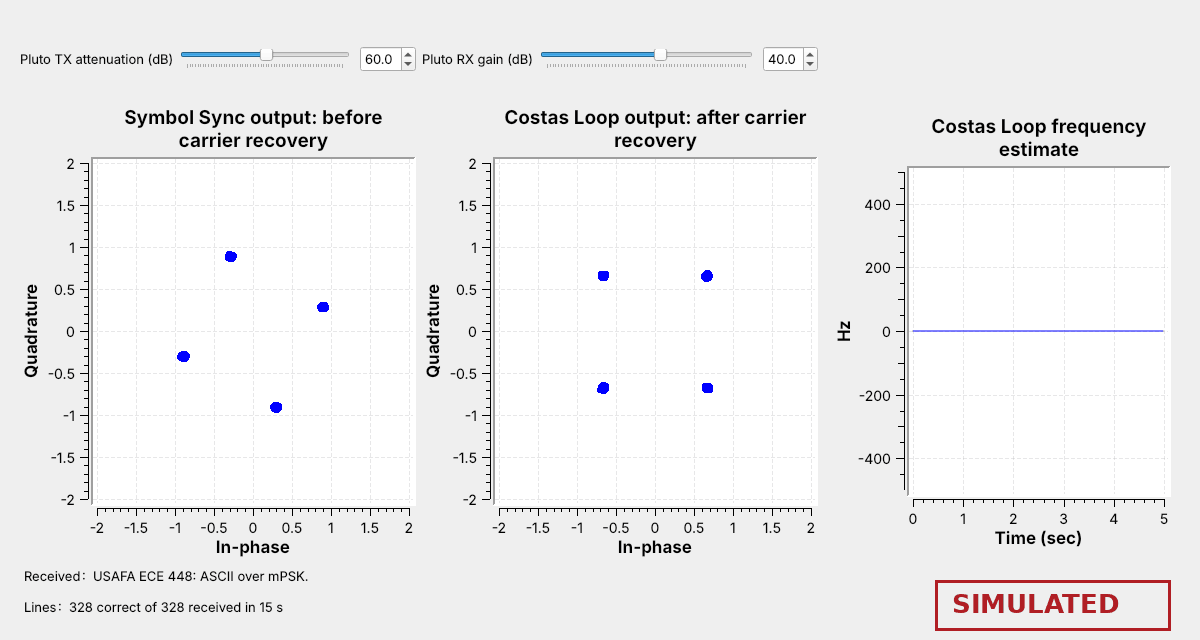
The figure is the PlutoSDR flowgraph run in simulation, with the Pluto Sink and Source replaced by a model of the cable using our estimate of the Pluto’s levels and noise. The real levels can differ, but the AGC should give the same picture. On the bench, look for the same three things: four tight clusters before and after the Costas Loop, a frequency estimate near 0 Hz, and lines arriving in the Lines label.
PlutoSDR Steps
With the Pluto unplugged, connect its TX port to its RX port with a short SMA cable and an inline 30 dB SMA attenuator. Do not connect an antenna, and do not connect the cable without the attenuator.
Plug the Pluto into USB and run
iio_info -sat the radioconda prompt; it should list a PlutoSDR context. The flowgraph uses the Pluto’s default address,ip:192.168.2.1.Open and run
L15-psk-pluto.grc. Within a few seconds the Costas Loop’s output should show four clusters and lines should arrive. If the clusters do not form, raise the RX gain a few dB at a time. Never set TX attenuation below 30 dB or change the slider’s range.Once lines arrive, screenshot the window for Question 7(a).
Stop and start the flowgraph three times with
diff= 1, and record whether text arrives each time. Then set the variablediffto 0 and stop and start it eight more times, recording whether text arrives each time, for Question 7(b). Setdiffback to 1, and stop and start the flowgraph.With
diff= 1, set the TX attenuation to 70, 80, and 89 dB in turn. At each, wait 30 s and record the Lines label for Question 7(c). Stop the flowgraph and unplug the Pluto before you disconnect the cable.
Part 3: After the Lab
Explain the order in which the constellations stopped delivering text.
Compare the 8PSK pull-in range with QPSK’s.
Explain the phases that decoded, and the Pluto runs.
The Writeup is Question 8, in three parts. Part (a) explains, in words, why the three constellations stopped delivering text in the order they did. Part (b) compares the 8PSK pull-in range with QPSK’s and asks what a link between two different PlutoSDRs would need before its Costas Loop. Part (c) explains which channel phases decoded, why the Pluto runs behaved as they did, and why real mPSK links use differential coding.
Lab Packet
L15-psk-link.grc: the whole mPSK text link with sliders for the noise amplitude, frequency offset, channel phase, and clock error, and a variable that turns differential coding on or off. No hardware needed.
L15-psk-pluto.grc: the link on one PlutoSDR, transmitting at 915 MHz into a cable from its TX port to its RX port through a 30 dB attenuator. Needs a PlutoSDR.
Looking Ahead
Lesson 16 hops the carrier from channel to channel.
Lesson 20 adds amplitude to the constellation with QAM.
Keep your carrier-recovery flowgraph and your tables. Lesson 16 turns to frequency hopping, where the transmitter moves its carrier many times a second and the receiver has to follow it. Lesson 20 returns to constellations: QAM varies the amplitude as well as the phase, so its receiver needs the same timing and carrier recovery as today’s, and an AGC that sets the level exactly.