# ECE 448
Software Defined Radios
## Lesson 3 — Signal Space
Spring 2027 · Dr. Neil Rogers

---
## Where We Were
- Lesson 2: a link closes when the received power clears the noise floor by the SNR the receiver needs
- The SDR display reads that SNR as the peak minus the floor
- What does the noise do to a digital signal?
Today: **a modulation is a set of points**, and noise decides how often the receiver picks the wrong one.
Note:
Open by putting the Lesson 2 ledger back on the screen and pointing at the noise floor. Today we look at what that noise does to the samples a receiver decides on. No error-rate formulas: we watch.
---
## Today's Plan
1. Three families: ASK/PAM, PSK, FSK
2. Binary PAM and the decision threshold
3. What noise does: antipodal and orthogonal signals
4. Basis functions and constellation diagrams
5. Decision regions, in GNU Radio and the constellation explorer
6. Gray coding, and reading a constellation in GNU Radio
Note:
The same order as the 2025 slides: binary PAM first, then constellations, then Gray coding.
---
## Three Families of Modulation
| Family | What changes per symbol | In this course |
| :-- | :-- | :-- |
| ASK / PAM | amplitude | Lessons 9 and 10 |
| PSK | phase | Lesson 15 |
| FSK | frequency | Lesson 8 |
$M$ choices per symbol carry $\log_2 M$ bits.
Note:
Two choices carry one bit, four carry two, eight carry three. "M-ary" means M choices. Each family gets its own flowgraph later in the course.
---
## Binary PAM
A 1 is a pulse at $+A$, a 0 a pulse at $-A$. Sample once per pulse and decide by sign.
Note:
The two pulses are the same shape with opposite signs, so they are antipodal. Zero, halfway between, is the decision threshold. GNU Radio's Binary Slicer is exactly this threshold, and Lesson 10 builds the receiver.
---
## Noise and the Threshold
As the SNR falls, the spreads widen, and more samples cross zero.
Note:
This replaces the 2025 probability-of-error derivation with the picture behind it. At 14 dB nothing comes near zero. At 4 dB the tails cross, and every red sample is a wrong bit. The threshold never moves; the samples just stray farther.
---
## Antipodal and Orthogonal
Same energy, same noise: the orthogonal points sit closer together, and more samples cross.
Note:
Binary FSK sends one of two tones, which are orthogonal, one per axis. Antipodal points are as far apart as the energy allows. That is why PAM and PSK get more out of the same power than FSK.
---
## Two Basis Functions
$$s(t) = I\cos(2\pi f_c t) - Q\sin(2\pi f_c t)$$
- Cosine and sine at the same frequency are orthogonal, so $I$ and $Q$ carry two independent numbers.
- Each symbol is a point $(I, Q)$; the two waveforms are its **basis functions**.
Note:
The SDR mixes with a cosine and a sine and hands GNU Radio the pair as one complex number. That is why every course SDR streams complex samples. Lesson 4 opens the hardware.
---
## Constellation Diagrams
PAM puts its points on a line, PSK on a circle; at the same energy, more points sit closer together.
Note:
Same transmitter power for all four; the dashed circle is that power. BPSK is 2-PAM on a carrier. QPSK and 4-PAM carry the same two bits, but QPSK uses both axes and keeps its points farther apart. 4-PAM comes back in Lesson 9 as a baseband signal.
---
## Noise and Decision Regions
The receiver picks the nearest point; for QPSK the decision regions are the quadrants.
Note:
QPSK at three SNRs. At 20 dB nothing crosses; at 10 dB a few do; at 4 dB the clouds overlap. Red is a sample in the wrong region. This is what the constellation sink shows, starting with the RDS receiver in Lesson 7.
---
## Try It in GNU Radio
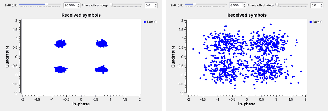 1. Open `L03-noise-constellation.grc` and run it.
2. Drag the SNR from 20 dB down to 6 dB.
3. Add a phase offset and watch the clouds rotate.
Note:
My demo; no SDR needed. Adapted from the GNU Radio wiki's QPSK Mod and Demod tutorial, its first half, without pulse shaping. Random Source, Chunks to Symbols with a Gray-coded QPSK table, and a Channel Model whose noise voltage comes from the SNR slider. Open Chunks to Symbols and show the symbol table: that list is the constellation.
---
## Constellation Explorer
- QPSK at 12 dB, then 8-PSK at 12 dB: the clouds reach the boundaries.
- Raise the SNR until 8-PSK is clean, then step up to 16-PSK.
- Add a phase offset to QPSK: the clouds rotate toward the boundaries.
↗ Interactive on the lesson page
Note:
Demo live. Let the class call out what they see as the SNR slider moves. End on the phase offset: past 45 degrees every symbol is in the wrong region with no noise at all, which motivates carrier recovery in Lesson 15.
---
## Gray Coding
- Each label differs from its neighbors by one bit.
- A slip to a neighbor then costs one bit, not three.
- Map it out for 8-PSK, starting from 000.
Note:
Hide the figure first and have them map out the 8-PSK Gray code, as in the 2025 slides. Then label it in natural binary and find the neighbors that differ in all three bits: 011 and 100. Every modulator we build uses a Gray code.
---
## Reading a Constellation in GNU Radio
Noise makes clouds, a phase offset rotates, a frequency offset spins into a ring, and a timing offset smears.
Note:
The constellation sink is the first place to look when a receiver fails. Lesson 9 fixes timing; Lesson 15 fixes phase and frequency. Each fix shows up as these shapes collapsing back into tight clouds.
---
## Key Point
A modulation is a set of points. Noise turns each point into a cloud, and a sample in a neighbor's region is a wrong decision. Points farther apart, or a higher SNR, keep the clouds in their own regions.
Note:
If they keep one picture, it is the noise clouds at three SNRs.
---
## Looking Ahead
- Lesson 4: the SDR hardware that turns a carrier into $I + jQ$
- Lesson 7: a constellation sink on a real signal
- Lessons 9, 10, and 15: PAM and PSK receivers built on these ideas
Note:
Before next time: sketch 2-PAM, 4-PAM, QPSK, and 8-PSK, mark their decision regions, and Gray-label 8-PSK.